## Data Flow Diagram: FairPFN Pre-training ### Overview The image is a data flow diagram illustrating the pre-training process of a FairPFN (Fair Prediction Function Network). It shows the generation of data, the input to a transformer, and the fair prediction process. The diagram is divided into three sections: data generation, transformer input, and fair prediction. ### Components/Axes * **Titles:** * a) Data generation * b) Transformer input * c) Fair prediction * Structural Causal Model (SCM) * Real-world Inference * Observational Dataset * FairPFN * Pre-training Loss * FairPFN Pre-training * **Variables/Labels:** * D: Dataset * A: Protected attribute (blue) * Xb: Biased observables (purple) * Yb: Biased outcome (orange) * Yf: Fair outcome (yellow) * U2: Unobserved variable (green) * X1, X2, X3: Observables (purple) * Dtrain: Training dataset * Dval: Inference set * Aval: Protected attribute in inference set * Xval: Observables in inference set * Ŷf: Predicted fair outcome (gray scale) * p(yf|xb, Db): Probability of fair outcome given biased observables and dataset * φ: Latent variable * p(yf|xb, φ): Probability of fair outcome given biased observables and latent variable * p(Db|φ): Probability of dataset given latent variable * p(φ): Probability of latent variable * **Diagram Elements:** * Structural Causal Model (SCM): A directed graph with nodes representing variables and edges representing causal relationships. * Observational Dataset: A table representing the dataset with columns for A, X1, X2, X3, and Yb. * FairPFN: A trapezoidal shape representing the Fair Prediction Function Network. * Pre-training Loss: Two columns representing the predicted fair outcome (Ŷf) and the fair outcome (Yf). * Arrows: Indicate the flow of data and processes. 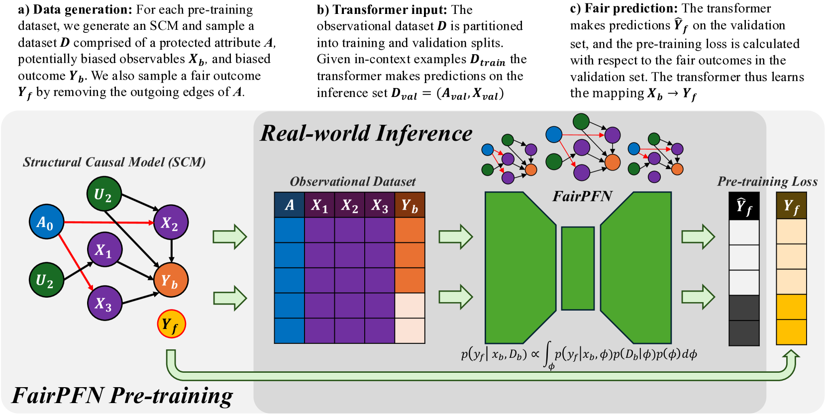### Detailed Analysis or Content Details **a) Data generation:** * Text: "For each pre-training dataset, we generate an SCM and sample a dataset D comprised of a protected attribute A, potentially biased observables Xb, and biased outcome Yb. We also sample a fair outcome Yf by removing the outgoing edges of A." * Structural Causal Model (SCM): * Nodes: A0 (blue), U2 (green, top), U2 (green, bottom), X1 (purple), X2 (purple), X3 (purple), Yb (orange), Yf (yellow, outlined in red). * Edges: * A0 -> X1 (red) * A0 -> X2 (red) * A0 -> X3 (red) * U2 -> X2 (black) * U2 -> Yb (black) * X1 -> Yb (black) * X2 -> Yb (black) * X3 -> Yb (black) **b) Transformer input:** * Text: "The observational dataset D is partitioned into training and validation splits. Given in-context examples Dtrain the transformer makes predictions on the inference set Dval = (Aval, Xval)" * Observational Dataset: * Columns: A (blue), X1 (purple), X2 (purple), X3 (purple), Yb (orange). * Rows: Four rows, each with a different shade of the column color. **c) Fair prediction:** * Text: "The transformer makes predictions Ŷf on the validation set, and the pre-training loss is calculated with respect to the fair outcomes in the validation set. The transformer thus learns the mapping Xb -> Yf" * FairPFN: A green trapezoid. * Pre-training Loss: * Ŷf (Predicted fair outcome): Four shades of gray, from black to white. * Yf (Fair outcome): Four shades of yellow/brown. * Formula: p(yf|xb, Db) ∝ ∫ p(yf|xb, φ)p(Db|φ)p(φ) dφ ### Key Observations * The diagram illustrates the process of generating a fair outcome (Yf) from a biased outcome (Yb) using a FairPFN. * The SCM shows the causal relationships between the variables. * The observational dataset represents the data used to train the FairPFN. * The FairPFN makes predictions on the validation set and calculates the pre-training loss. ### Interpretation The diagram describes a method for mitigating bias in machine learning models. The process starts with a structural causal model that represents the relationships between variables, including a protected attribute (A) and a biased outcome (Yb). The FairPFN is trained to predict a fair outcome (Yf) by learning the mapping from biased observables (Xb) to Yf. The pre-training loss is calculated with respect to the fair outcomes, ensuring that the model learns to predict fair outcomes. The formula represents the probability of the fair outcome given the biased observables and dataset, which is proportional to the integral of the product of the probabilities of the fair outcome given the biased observables and latent variable, the dataset given the latent variable, and the latent variable. This approach aims to remove the influence of the protected attribute on the outcome, resulting in a fairer prediction.

\n ## Diagram: FairPFN Pre-training Pipeline ### Overview This diagram illustrates the pre-training pipeline for FairPFN, a model designed for real-world inference with a focus on fairness. The pipeline consists of three main stages: data generation, transformer input, fair prediction, and then a visual representation of the process using a Structural Causal Model (SCM), an Observational Dataset, the FairPFN model itself, and the calculation of a pre-training loss. ### Components/Axes The diagram is segmented into four main sections: 1. **Data Generation (a):** Describes the process of creating the dataset. 2. **Transformer Input (b):** Explains how the observational dataset is used as input to a transformer model. 3. **Fair Prediction (c):** Details the prediction process and loss calculation. 4. **Real-world Inference:** A visual representation of the pipeline with the SCM, Observational Dataset, FairPFN, and Pre-training Loss. The key elements within the "Real-world Inference" section are: * **Structural Causal Model (SCM):** Nodes labeled A₀, U₂, X₁, X₂, X₃, Yb, and Yf, with directed edges representing causal relationships. * **Observational Dataset:** A table with columns A, X₁, X₂, X₃, and Yb. * **FairPFN:** A complex network of interconnected nodes. * **Pre-training Loss:** Represented by the symbols Ŷf and Yf. ### Detailed Analysis or Content Details **a) Data Generation:** * A dataset is generated comprising a protected attribute *A*, potentially biased observables *Xb*, and biased outcome *Yb*. * A fair outcome *Yf* is sampled by removing the outgoing edges of *A*. **b) Transformer Input:** * The observational dataset *D* is partitioned into training and validation splits. * Given in-context examples *Dtrain*, the transformer makes predictions on the inference set *Dval* = (*Aval*, *Xval*). **c) Fair Prediction:** * The transformer makes predictions Ŷf on the validation set. * The pre-training loss is calculated with respect to the fair outcomes in the validation set. * The transformer learns the mapping *Xb* → *Yf*. **Real-world Inference - SCM:** * The SCM shows causal relationships: * U₂ influences X₁, X₂, and X₃. * A₀ influences X₁. * X₁, X₂, and X₃ influence Yb. * Yb influences Yf. **Real-world Inference - Observational Dataset:** * The dataset table has 5 columns: A, X₁, X₂, X₃, and Yb. * The table is filled with a heatmap-like color gradient. The colors range from dark blue to dark red, indicating varying values. It's difficult to extract precise numerical values from the color gradient without a legend, but the color intensity suggests a range of values. * The table appears to have approximately 10-15 rows. **Real-world Inference - FairPFN:** * The FairPFN is a complex network of interconnected nodes. The nodes are colored in shades of green and purple. * The network has multiple layers and connections. **Real-world Inference - Pre-training Loss:** * Ŷf (predicted fair outcome) is connected to Yf (fair outcome). * The arrow indicates the calculation of the pre-training loss. **Mathematical Formula:** * p(*Yf* | *Xb*, *Db*) ∝ ∫ p(*Yf* | *Xb*, φ)p(*D♭* | φ) dφ ### Key Observations * The diagram emphasizes the importance of fairness by explicitly generating a "fair outcome" (*Yf*) and using it for loss calculation. * The SCM visually represents the causal relationships between variables, highlighting the potential for bias introduced by the protected attribute *A*. * The heatmap-like representation of the observational dataset suggests that the data is high-dimensional and potentially complex. * The FairPFN model is a complex neural network, likely designed to capture intricate relationships in the data. ### Interpretation The diagram illustrates a pipeline for training a fair machine learning model. The core idea is to mitigate bias by explicitly modeling the causal relationships between variables and using a "fair outcome" as the target for training. The SCM provides a visual representation of these relationships, while the observational dataset provides the data for training. The FairPFN model learns to predict the fair outcome, and the pre-training loss ensures that the model is aligned with the desired fairness criteria. The mathematical formula suggests a probabilistic approach to fairness, where the model aims to estimate the probability of the fair outcome given the observed data. The use of a transformer model suggests that the pipeline is designed to handle sequential or contextual data. The diagram suggests a sophisticated approach to fairness that goes beyond simply removing the protected attribute from the training data. It attempts to address the underlying causal mechanisms that lead to bias.

## Diagram: FairPFN Pre-training Framework ### Overview This image is a technical diagram illustrating the pre-training framework for a model called "FairPFN." The diagram is divided into three sequential stages (a, b, c) at the top, which describe the process, and a larger visual flow below that maps these stages to a "Real-world Inference" pipeline. The overall purpose is to show how a Structural Causal Model (SCM) is used to generate data for training a transformer model (FairPFN) to make fair predictions by learning to map biased observables to fair outcomes. ### Components/Axes The diagram is segmented into several key components: 1. **Top Text Blocks (Process Description):** * **a) Data generation:** Describes generating an SCM and sampling a dataset `D` with a protected attribute `A`, biased observables `X_b`, and biased outcome `Y_b`. A fair outcome `Y_f` is also sampled by removing outgoing edges from `A`. * **b) Transformer input:** Describes partitioning the observational dataset `D` into training and validation splits. The transformer uses in-context examples `D_train` to make predictions on the inference set `D_val = (A_val, X_val)`. * **c) Fair prediction:** Describes the transformer making predictions `Ŷ_f` on the validation set. The pre-training loss is calculated with respect to the fair outcomes `Y_f`, teaching the model the mapping `X_b → Y_f`. 2. **Main Visual Flow (Left to Right):** * **Left: Structural Causal Model (SCM):** A directed acyclic graph with nodes and arrows. * **Nodes:** `A0` (blue circle), `U2` (green circle, appears twice), `X1`, `X2`, `X3` (purple circles), `Y_b` (orange circle), `Y_f` (yellow circle with red outline). * **Arrows:** Black arrows indicate causal relationships. Red arrows originate from `A0` and point to `X2` and `X3`, indicating a biased or protected attribute's influence. * **Center-Left: Observational Dataset:** A table with columns labeled `A` (blue header), `X1`, `X2`, `X3` (purple headers), and `Y_b` (orange header). The table contains 5 rows of colored cells (blue, purple, orange, light beige) representing data samples. * **Center: FairPFN:** A large, green, abstract block diagram representing the transformer model. Above it are three small copies of the SCM graph. Below it is a mathematical equation: `p(y_f | x_b, D_b) ∝ ∫_φ p(y_f | x_b, φ) p(D_b | φ) p(φ) dφ`. * **Center-Right: Pre-training Loss:** Two vertical bars. * Left bar: Labeled `Ŷ_f` (predicted fair outcome), with a grayscale gradient from white (top) to black (bottom). * Right bar: Labeled `Y_f` (true fair outcome), with a color gradient from light beige (top) to yellow (bottom). * **Arrows:** Large, light green arrows show the data flow from the SCM to the dataset, from the dataset to FairPFN, and from FairPFN to the loss calculation. A final green arrow loops from the loss back to the SCM, indicating the pre-training cycle. 3. **Title:** The entire lower section is titled "**FairPFN Pre-training**" in a large, bold, serif font. ### Detailed Analysis * **SCM Node Relationships:** * `A0` has direct red arrows to `X2` and `X3`. * `U2` (top) has arrows to `X1` and `Y_b`. * `U2` (bottom) has an arrow to `X1`. * `X1` has arrows to `X2` and `Y_b`. * `X2` has an arrow to `Y_b`. * `X3` has an arrow to `Y_b`. * `Y_f` is shown as a separate node, derived from the SCM by "removing the outgoing edges of A" as per the text in (a). * **Data Flow & Process Mapping:** 1. The **SCM** (Stage a) is used to generate the **Observational Dataset**. 2. The dataset is fed into the **FairPFN** model (Stages b & c). 3. The model produces predictions `Ŷ_f`. 4. The **Pre-training Loss** is computed by comparing `Ŷ_f` to the true fair outcome `Y_f`. 5. The loss is used to update the model, completing the pre-training loop. * **Mathematical Equation:** The equation below FairPFN expresses the model's predictive distribution as a proportionality (`∝`) involving an integral over model parameters `φ`. It combines the likelihood of the fair outcome given the biased input and parameters, the likelihood of the biased data given the parameters, and a prior over the parameters. ### Key Observations * **Color Coding is Systematic:** Blue is consistently used for the protected attribute `A`. Purple is used for the observables `X1, X2, X3`. Orange represents the biased outcome `Y_b`. Yellow represents the fair outcome `Y_f`. * **Bias Representation:** The red arrows from `A0` in the SCM visually highlight the pathways of bias that the framework aims to remove to achieve `Y_f`. * **Model Abstraction:** The FairPFN is represented as a generic green block, emphasizing its role as a black-box transformer model within this causal framework. * **Loss Visualization:** The loss bars visually contrast the model's grayscale predictions (`Ŷ_f`) against the colored true fair targets (`Y_f`), implying the goal is to align the prediction distribution with the fair outcome distribution. ### Interpretation This diagram outlines a methodology for instilling fairness into a predictive model through causal pre-training. The core idea is to use a known or assumed causal structure (the SCM) to generate synthetic data where the direct effect of a protected attribute (`A`) on the outcome is removed, creating a "fair" target (`Y_f`). A transformer model (FairPFN) is then trained not on the real-world biased outcome (`Y_b`), but on this constructed fair outcome. The process is "pre-training" because it happens before the model is applied to real-world tasks. By learning the mapping from biased observables (`X_b`) to fair outcomes (`Y_f`) in a controlled, causal environment, the model is intended to internalize a fair prediction rule. The integral in the equation suggests a Bayesian approach, marginalizing over model parameters to make predictions. The framework implies that real-world inference (using the pre-trained model) will then produce fair predictions even when only biased data is available, as the model has learned to "ignore" the biased pathways from `A`. The key assumption is the validity of the initial SCM used for data generation.

## Diagram: FairPFN Pre-training Process for Fair Prediction ### Overview The diagram illustrates a technical workflow for training a fair prediction model (FairPFN) using structural causal models (SCM) and observational data. It emphasizes fairness constraints through pre-training loss calculations that compare model predictions against protected attributes and fair outcomes. ### Components/Axes 1. **Structural Causal Model (SCM)** - Leftmost section with nodes: - Protected attribute: `A₀` (blue) - Unobserved confounders: `U₂` (green) - Observables: `X₁`, `X₂`, `X₃` (purple) - Biased outcome: `Y_b` (orange) - Fair outcome: `Y_f` (yellow) - Arrows indicate causal relationships (e.g., `A₀ → X₂`, `U₂ → X₁`). 2. **Observational Dataset** - Tabular format with columns: - `A` (protected attribute, blue) - `X₁`, `X₂`, `X₃` (observables, purple) - `Y_b` (biased outcome, orange) - Color-coded cells suggest data distribution (e.g., darker purple for `X₁`). 3. **FairPFN** - Central green block representing the model architecture. - Equations: - `p(y_f | x_b, D_b) ∝ ∫ p(y_f | x_b, φ)p(D_b | φ)p(φ)dφ` - Indicates probabilistic inference over fairness parameters (φ). 4. **Pre-training Loss** - Rightmost section with two columns: - `Ŷ_f` (model predictions, black bars) - `Y_f` (fair outcomes, yellow bars) - Visual comparison of prediction accuracy vs. fairness targets. ### Detailed Analysis - **SCM to Observational Dataset**: The SCM generates a dataset `D` with protected attribute `A`, observables `X_b`, and biased outcome `Y_b`. A fair outcome `Y_f` is derived by removing edges from `A`. - **Transformer Input**: The observational dataset is split into training (`D_train`) and validation (`D_val`) sets. The transformer maps `X_b → Y_f` using in-context examples. - **Fair Prediction**: The transformer makes predictions `Ŷ_f` on the validation set. Pre-training loss is calculated by comparing `Ŷ_f` to `Y_f`, ensuring alignment with fairness constraints. ### Key Observations 1. **Causal Structure**: - Protected attribute `A₀` influences observables `X_b` via confounders `U₂`, creating potential bias in `Y_b`. - Fair outcome `Y_f` isolates `X_b` from `A₀` to mitigate bias. 2. **Data Representation**: - Observational dataset uses color gradients to differentiate data types (e.g., blue for `A`, orange for `Y_b`). - Pre-training loss bars show a direct comparison between model outputs (`Ŷ_f`) and ground truth (`Y_f`). 3. **Mathematical Formulation**: - The FairPFN integrates fairness constraints via probabilistic inference over parameters `φ`, balancing prediction accuracy and fairness. ### Interpretation This workflow demonstrates a fairness-aware machine learning pipeline. By explicitly modeling causal relationships (SCM) and incorporating fairness constraints into the loss function, the model aims to reduce bias in predictions. The pre-training loss acts as a regularization term, penalizing deviations from fair outcomes. The use of observational data with protected attributes highlights challenges in real-world deployment, where unobserved confounders (`U₂`) may still influence fairness. The diagram emphasizes the importance of causal reasoning in designing robust, equitable AI systems.