## Log-Log Plot: Gradient Updates vs. Dimension ### Overview The image is a log-log plot showing the relationship between gradient updates and dimension for different values of epsilon (ε*). The plot includes data points with error bars and linear fits for each epsilon value. The x and y axes are both on a logarithmic scale. ### Components/Axes * **X-axis:** Dimension (log scale), with tick marks at 4 x 10¹, 6 x 10¹, 10², and 2 x 10². * **Y-axis:** Gradient updates (log scale), with tick marks at 10³ and 10⁴. * **Legend (top-left):** * Blue dashed line: Linear fit: slope = 1.4451 * Green dashed line: Linear fit: slope = 1.4692 * Red dashed line: Linear fit: slope = 1.5340 * Blue circle with error bars: ε* = 0.008 * Green square with error bars: ε* = 0.01 * Red triangle with error bars: ε* = 0.012 ### Detailed Analysis * **ε* = 0.008 (Blue Circles):** * Trend: The data points generally slope upward. * Data points (approximate): * Dimension = 40, Gradient updates ≈ 450 ± 50 * Dimension = 60, Gradient updates ≈ 700 ± 50 * Dimension = 100, Gradient updates ≈ 1300 ± 100 * Dimension = 200, Gradient updates ≈ 4000 ± 1000 * **ε* = 0.01 (Green Squares):** * Trend: The data points generally slope upward. * Data points (approximate): * Dimension = 40, Gradient updates ≈ 350 ± 50 * Dimension = 60, Gradient updates ≈ 650 ± 50 * Dimension = 100, Gradient updates ≈ 1200 ± 100 * Dimension = 200, Gradient updates ≈ 4500 ± 500 * **ε* = 0.012 (Red Triangles):** * Trend: The data points generally slope upward. * Data points (approximate): * Dimension = 40, Gradient updates ≈ 300 ± 50 * Dimension = 60, Gradient updates ≈ 550 ± 50 * Dimension = 100, Gradient updates ≈ 1000 ± 100 * Dimension = 200, Gradient updates ≈ 3000 ± 500 * **Linear Fits:** * Blue dashed line (ε* = 0.008): Linear fit with slope = 1.4451 * Green dashed line (ε* = 0.01): Linear fit with slope = 1.4692 * Red dashed line (ε* = 0.012): Linear fit with slope = 1.5340 ### Key Observations * All three data series (ε* = 0.008, 0.01, and 0.012) show a positive correlation between dimension and gradient updates. As the dimension increases, the number of gradient updates also increases. * The slopes of the linear fits are all close to each other, ranging from 1.4451 to 1.5340. * The data points for higher epsilon values (ε* = 0.01 and 0.012) tend to have slightly lower gradient updates compared to the data points for lower epsilon values (ε* = 0.008) at the same dimension. * The error bars appear to increase with dimension, suggesting greater variability in gradient updates at higher dimensions. ### Interpretation The plot suggests that the number of gradient updates required increases with the dimension of the problem. The linear fits indicate a power-law relationship between dimension and gradient updates, with the slopes representing the exponents of this relationship. The different epsilon values seem to influence the magnitude of gradient updates, with higher epsilon values potentially leading to slightly lower gradient updates for a given dimension. The increasing error bars at higher dimensions could indicate that the relationship becomes less stable or more sensitive to other factors as the dimension increases.

\n ## Chart: Gradient Updates vs. Dimension (Log Scale) ### Overview The image presents a chart illustrating the relationship between gradient updates (on a logarithmic scale) and dimension (also on a logarithmic scale). Three different data series are plotted, each representing a different value of ε* (epsilon star). Each data point includes error bars, and linear fits are shown for each series. ### Components/Axes * **X-axis:** Dimension (log scale), ranging from approximately 4 x 10¹ to 2 x 10². Axis markers are at 40, 60, 100, and 200. * **Y-axis:** Gradient updates (log scale), ranging from approximately 10³ to 10⁴. Axis markers are at 1000 and 10000. * **Legend:** Located in the top-left corner. * Blue line with circular markers: ε* = 0.008, Linear fit: slope = 1.4451 * Green line with triangular markers: ε* = 0.01, Linear fit: slope = 1.4692 * Red line with inverted triangular markers: ε* = 0.012, Linear fit: slope = 1.5340 * **Grid:** A grid is present on the chart to aid in reading values. ### Detailed Analysis The chart displays three data series, each showing an upward trend. The trend is approximately linear, as indicated by the linear fit lines. Error bars are present for each data point, indicating the uncertainty in the measurements. **Data Series 1 (ε* = 0.008 - Blue):** * At Dimension = 40, Gradient Updates ≈ 1800 (with error bars extending roughly from 1500 to 2100). * At Dimension = 60, Gradient Updates ≈ 2600 (with error bars extending roughly from 2200 to 3000). * At Dimension = 100, Gradient Updates ≈ 4000 (with error bars extending roughly from 3500 to 4500). * At Dimension = 200, Gradient Updates ≈ 7500 (with error bars extending roughly from 6500 to 8500). **Data Series 2 (ε* = 0.01 - Green):** * At Dimension = 40, Gradient Updates ≈ 2000 (with error bars extending roughly from 1700 to 2300). * At Dimension = 60, Gradient Updates ≈ 2800 (with error bars extending roughly from 2400 to 3200). * At Dimension = 100, Gradient Updates ≈ 4300 (with error bars extending roughly from 3800 to 4800). * At Dimension = 200, Gradient Updates ≈ 8000 (with error bars extending roughly from 7000 to 9000). **Data Series 3 (ε* = 0.012 - Red):** * At Dimension = 40, Gradient Updates ≈ 2200 (with error bars extending roughly from 1900 to 2500). * At Dimension = 60, Gradient Updates ≈ 3100 (with error bars extending roughly from 2700 to 3500). * At Dimension = 100, Gradient Updates ≈ 4800 (with error bars extending roughly from 4300 to 5300). * At Dimension = 200, Gradient Updates ≈ 9000 (with error bars extending roughly from 8000 to 10000). ### Key Observations * All three data series exhibit a positive correlation between dimension and gradient updates. * The slope of the linear fit increases with increasing ε*. This suggests that larger values of ε* require more gradient updates for a given dimension. * The error bars indicate a significant degree of variability in the gradient updates, particularly at higher dimensions. * The red line (ε* = 0.012) consistently shows the highest gradient updates for any given dimension. ### Interpretation The chart demonstrates that the number of gradient updates required to train a model increases with the dimensionality of the input data. The rate of increase (the slope of the linear fit) is influenced by the value of ε*. A larger ε* leads to a steeper slope, indicating a greater sensitivity to dimensionality. This could be related to the difficulty of optimizing the model in higher-dimensional spaces, requiring more iterations (gradient updates) to converge. The error bars suggest that the relationship is not perfectly linear and that there is inherent noise or variability in the training process. The consistent ordering of the lines (red > green > blue) suggests that ε* is a significant factor in determining the computational cost of training. The logarithmic scales used for both axes suggest that the relationship may be exponential or power-law in nature, and the linear fits are approximations over the observed range of dimensions.

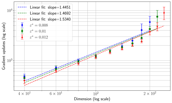
## Log-Log Scatter Plot with Linear Fits: Gradient Updates vs. Dimension ### Overview The image is a scientific chart, specifically a log-log scatter plot with error bars and overlaid linear regression lines. It illustrates the relationship between the dimension of a problem (x-axis) and the number of gradient updates required (y-axis) for three different values of a parameter denoted as ε* (epsilon star). The plot demonstrates a power-law scaling relationship. ### Components/Axes * **Chart Type:** Log-log scatter plot with linear fits. * **X-Axis:** * **Label:** "Dimension (log scale)" * **Scale:** Logarithmic. * **Major Tick Markers:** `4 × 10¹`, `6 × 10¹`, `10²`, `2 × 10²`. These correspond to the numerical values 40, 60, 100, and 200. * **Y-Axis:** * **Label:** "Gradient updates (log scale)" * **Scale:** Logarithmic. * **Major Tick Markers:** `10³`, `10⁴`. These correspond to the numerical values 1000 and 10,000. * **Legend (Position: Top-Left Corner):** * **Linear Fit Entries (Dashed Lines):** * Blue dashed line: "Linear fit: slope=1.4451" * Green dashed line: "Linear fit: slope=1.4692" * Red dashed line: "Linear fit: slope=1.5340" * **Data Series Entries (Points with Error Bars):** * Blue circle marker: "ε* = 0.008" * Green square marker: "ε* = 0.01" * Red triangle marker: "ε* = 0.012" * **Grid:** A light gray grid is present, aligned with the major tick marks on both axes. ### Detailed Analysis **Data Series and Trends:** 1. **Blue Series (ε* = 0.008):** * **Visual Trend:** The data points (blue circles) follow a clear upward linear trend on the log-log plot. The associated blue dashed linear fit line has a slope of 1.4451. * **Data Points (Approximate from visual inspection):** * At Dimension ~40: Gradient updates ~300 * At Dimension ~60: Gradient updates ~600 * At Dimension ~100: Gradient updates ~1,200 * At Dimension ~200: Gradient updates ~4,000 * **Error Bars:** The vertical error bars (representing uncertainty or variance) are relatively small for lower dimensions and increase moderately with dimension. 2. **Green Series (ε* = 0.01):** * **Visual Trend:** The data points (green squares) also follow a strong upward linear trend, slightly steeper than the blue series. The green dashed linear fit line has a slope of 1.4692. * **Data Points (Approximate):** * At Dimension ~40: Gradient updates ~350 * At Dimension ~60: Gradient updates ~700 * At Dimension ~100: Gradient updates ~1,500 * At Dimension ~200: Gradient updates ~5,500 * **Error Bars:** Error bars are larger than those for the blue series at corresponding dimensions, indicating greater variance. 3. **Red Series (ε* = 0.012):** * **Visual Trend:** The data points (red triangles) show the steepest upward linear trend of the three series. The red dashed linear fit line has the highest slope of 1.5340. * **Data Points (Approximate):** * At Dimension ~40: Gradient updates ~400 * At Dimension ~60: Gradient updates ~800 * At Dimension ~100: Gradient updates ~1,800 * At Dimension ~200: Gradient updates ~7,000 * **Error Bars:** This series exhibits the largest error bars, which grow significantly with dimension, suggesting the highest variability in the number of updates required. **Linear Fits:** All three linear fits (dashed lines) align well with their respective data series, confirming the power-law relationship: `Gradient updates ∝ (Dimension)^slope`. The slope increases with ε*. ### Key Observations 1. **Consistent Scaling Law:** All three data series exhibit a linear relationship on the log-log plot, indicating a power-law scaling between problem dimension and computational cost (gradient updates). 2. **Slope Increases with ε*:** The slope of the linear fit increases from 1.4451 (ε*=0.008) to 1.5340 (ε*=0.012). This means the required gradient updates grow *super-linearly* with dimension, and the rate of this super-linear growth is higher for larger values of ε*. 3. **Variance Increases with ε* and Dimension:** The size of the error bars increases both with the parameter ε* and with the dimension. The red series (ε*=0.012) at the highest dimension (200) shows the largest uncertainty. 4. **Absolute Values:** For any given dimension, a larger ε* value results in a higher number of gradient updates. For example, at dimension 200, the updates range from ~4,000 (ε*=0.008) to ~7,000 (ε*=0.012). ### Interpretation This chart likely comes from the field of optimization or machine learning, analyzing the convergence rate of an algorithm (e.g., for training a model or solving a high-dimensional problem). * **What the data suggests:** The number of iterations (gradient updates) needed for the algorithm to converge scales as a power law with the problem's dimensionality. The exponent of this power law (the slope) is greater than 1, meaning the problem becomes disproportionately harder as dimension increases. * **Role of ε*:** The parameter ε* appears to be a tolerance or step-size related parameter. A larger ε* (0.012 vs. 0.008) leads to: 1. **More updates needed** (higher y-values), suggesting a more conservative or precise convergence criterion. 2. **A steeper scaling slope**, meaning the penalty for increasing dimension is more severe. 3. **Greater variability** in the number of updates required, as shown by the larger error bars. This could imply that with a larger ε*, the algorithm's performance becomes more sensitive to the specific instance of the problem at a given dimension. * **Practical Implication:** The chart provides a quantitative model for predicting computational cost. If one knows the dimension of their problem and chooses a tolerance ε*, they can estimate the expected number of gradient updates and the associated uncertainty. The super-linear scaling (slope > 1) is a critical consideration for scalability, warning that simply doubling the dimension will more than double the required computational effort.

## Line Chart: Gradient Updates vs. Dimension (Log-Log Scale) ### Overview The chart illustrates the relationship between **dimension** (log scale) and **gradient updates** (log scale) across three distinct linear fits, each associated with a specific slope and ε* value. Three data series are plotted, with markers and error bars indicating variability in gradient updates for different ε* values. --- ### Components/Axes - **X-axis**: "Dimension (log scale)" ranging from $4 \times 10^1$ to $2 \times 10^2$. - **Y-axis**: "Gradient updates (log scale)" ranging from $10^3$ to $10^4$. - **Legend**: Located in the **top-left corner**, with three entries: - **Blue dashed line**: Slope = 1.4451, ε* = 0.008. - **Green dash-dot line**: Slope = 1.4692, ε* = 0.01. - **Red dotted line**: Slope = 1.5340, ε* = 0.012. - **Data Points**: - Blue circles (ε* = 0.008). - Green squares (ε* = 0.01). - Red triangles (ε* = 0.012). - **Error Bars**: Vertical error bars on data points indicate uncertainty in gradient updates. --- ### Detailed Analysis 1. **Blue Line (Slope = 1.4451, ε* = 0.008)**: - Data points (blue circles) align closely with the dashed line. - At $4 \times 10^1$ dimension, gradient updates ≈ $10^3$. - At $2 \times 10^2$ dimension, gradient updates ≈ $10^4$. - Error bars suggest moderate variability (e.g., ±10% at $10^4$ updates). 2. **Green Line (Slope = 1.4692, ε* = 0.01)**: - Data points (green squares) follow the dash-dot line. - At $4 \times 10^1$ dimension, gradient updates ≈ $10^3$. - At $2 \times 10^2$ dimension, gradient updates ≈ $10^4$. - Error bars are slightly larger than the blue line, indicating higher uncertainty. 3. **Red Line (Slope = 1.5340, ε* = 0.012)**: - Data points (red triangles) align with the dotted line. - At $4 \times 10^1$ dimension, gradient updates ≈ $10^3$. - At $2 \times 10^2$ dimension, gradient updates ≈ $10^4$. - Error bars are the largest, suggesting greater variability at higher ε*. --- ### Key Observations - **Trend**: All three lines exhibit a **positive power-law relationship** between dimension and gradient updates, with steeper slopes for higher ε* values. - **Consistency**: Data points for each ε* value closely follow their respective linear fits, confirming the power-law scaling. - **Outliers**: No significant outliers; all data points fall within error margins. - **Slope Correlation**: Higher ε* values (0.012) correspond to steeper slopes (1.5340), suggesting a direct relationship between learning rate and update scaling. --- ### Interpretation The chart demonstrates that **gradient updates scale polynomially with dimension**, with the exponent (slope) increasing as ε* increases. This implies: - **Higher learning rates (ε*)** require more gradient updates to achieve convergence in higher-dimensional spaces. - The **power-law relationship** highlights the computational cost of training in high-dimensional settings, where updates grow faster than linearly with dimension. - The error bars indicate that variability in gradient updates increases with ε*, possibly due to instability in optimization at larger learning rates. This analysis underscores the trade-off between learning rate and computational efficiency in high-dimensional optimization problems.