TECHNICAL ASSET FINGERPRINT
24c2228d0fc8a303e60e9a40
Click to view fullscreen
Press ESC or click to close
FOUND IN PAPERS
EXPERT: healer-alpha-free VERSION 1
RUNTIME: free/openrouter/healer-alpha
INTEL_VERIFIED
## Diagram: Interdisciplinary Applications of Machine Learning in Physics
### Overview
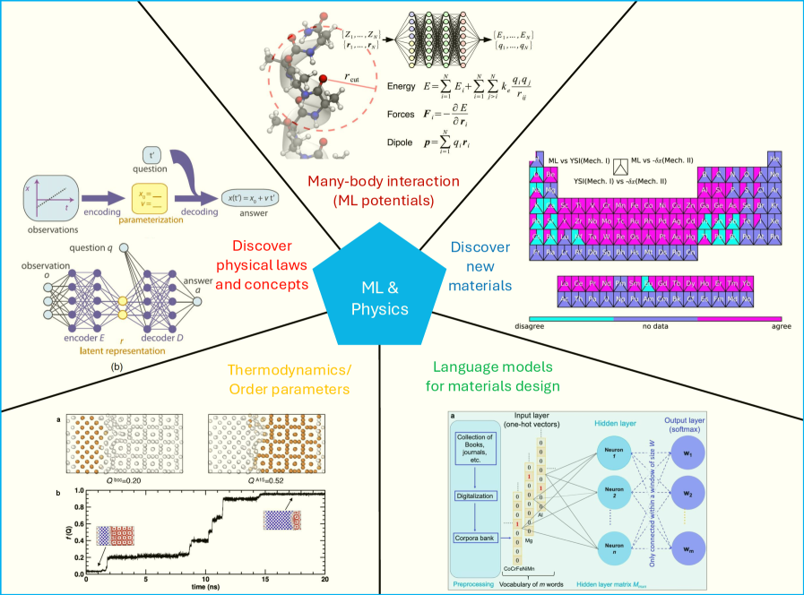
This image is a conceptual infographic illustrating five key research areas at the intersection of Machine Learning (ML) and Physics. A central blue hexagon labeled "ML & Physics" connects to five surrounding thematic blocks, each containing specific diagrams, equations, and data visualizations. The overall layout is a radial diagram with a light beige background.
### Components/Axes
The diagram is segmented into five primary regions radiating from the center:
1. **Top-Center:** "Many-body interaction (ML potentials)"
2. **Top-Right:** "Discover new materials"
3. **Bottom-Right:** "Language models for materials design"
4. **Bottom-Left:** "Thermodynamics/Order parameters"
5. **Top-Left:** "Discover physical laws and concepts"
A secondary, smaller diagram labeled "(b)" is nested within the "Discover physical laws and concepts" section.
### Detailed Analysis
#### 1. Many-body interaction (ML potentials)
* **Visual:** A molecular structure (ball-and-stick model) with atoms in red, blue, and white. A dashed red circle highlights an interaction radius `r_cut`.
* **Equations:** To the right of the molecule, three equations are presented:
* **Energy:** `E = Σ_i E_i + Σ_i Σ_j>k k_e * (q_i * q_j)/r_ij`
* **Forces:** `F_i = - ∂E/∂r_i`
* **Dipole:** `p = Σ_i q_i * r_i`
* **Neural Network Diagram:** Above the equations, a schematic shows a neural network processing coordinates `{Z_1,...,Z_N}` and distances `{r_1,...,r_N}` to output energies `{E_1,...,E_N}` and charges `{q_1,...,q_N}`.
#### 2. Discover new materials
* **Visual:** A large, complex heatmap or comparison matrix. The matrix is composed of many small triangular cells.
* **Legend:** Located at the bottom of this section. It defines a color scale:
* **Purple/Magenta:** "disagree"
* **Grey:** "no data"
* **Cyan/Teal:** "agree"
* **Matrix Labels:** The matrix is divided into sections with text labels:
* Top-left block: "ML vs YSI(Mech. II)"
* Top-right block: "ML vs -ln(Mech. II)"
* Bottom block: "YSI(Mech. II) vs -ln(Mech. II)"
* **Data Trend:** The matrix shows a patchwork of colors. The "ML vs YSI" block has significant areas of both "agree" (cyan) and "disagree" (purple). The "ML vs -ln" block is predominantly "agree" (cyan). The "YSI vs -ln" block is almost entirely "disagree" (purple).
#### 3. Language models for materials design
* **Visual:** A schematic of a neural network architecture.
* **Components (Left to Right):**
* **Input:** "Collection of Books, patents, etc." -> "Digitization" -> "Corpora bank" -> "Preprocessing" -> "Vocabulary of M words".
* **Network Layers:**
* "Input layer (one-hot vectors)": Shows a vertical vector of 0s and a single 1.
* "Hidden layer": Contains circles labeled "Neuron 1", "Neuron 2", ..., "Neuron N". Connections are labeled "Only connected with window of k W".
* "Output layer (softmax)": Contains circles labeled "W_1", "W_2", ..., "W_M".
* **Text Annotations:** "CoD/PtNiAl" is written near the input. "Hidden layer matrix M_h" is noted below the hidden layer.
#### 4. Thermodynamics/Order parameters
* **Visual (Top):** Two lattice diagrams labeled **a**.
* Left lattice: Disordered arrangement of brown and white circles. Label: `Q^M=0.20`.
* Right lattice: Ordered, checkerboard-like arrangement. Label: `Q^M=0.52`.
* **Visual (Bottom):** A line graph labeled **b**.
* **Y-axis:** Label is `Q^M`. Scale runs from 0.0 to 1.0 with increments of 0.2.
* **X-axis:** Label is `time [ns]`. Scale runs from 0 to 20 with increments of 5.
* **Data Trend:** The black line shows `Q^M` starting near 0, rising sharply around 2 ns to ~0.4, plateauing, then rising again around 12 ns to a final plateau near 0.9. Two small lattice insets are placed on the graph, corresponding to the low-order (start) and high-order (end) states.
#### 5. Discover physical laws and concepts
* **Main Diagram:** A flowchart showing a process from "observations" to "answer".
* **Steps:** "observations" (graph of `x` vs `t`) -> "encoding" -> "parameterization" (box with `x_0`, `v`) -> "decoding" -> "answer" (`x(t) = x_0 + v*t`).
* **Question:** A "question" input (box with `t*`) feeds into the parameterization step.
* **Sub-diagram (b):** A detailed neural network architecture.
* **Components:** "observation o" (input layer), "encoder E", "latent representation" (bottleneck layer), "decoder D", "answer a" (output layer).
* **Question Flow:** A "question q" is shown as a separate input that interacts with the latent representation.
### Key Observations
1. **Interdisciplinary Flow:** The diagram explicitly connects abstract ML concepts (encoders, decoders, neural networks) to concrete physical outputs (molecular energies, material properties, thermodynamic order parameters, symbolic equations).
2. **Data Representation:** Different physical problems require different data representations: 3D coordinates for molecules, text corpora for materials design, lattice configurations for thermodynamics, and time-series observations for law discovery.
3. **Validation Methods:** The "Discover new materials" section highlights a key challenge in computational science: comparing predictions from different models (ML, YSI, -ln) and visualizing areas of agreement and disagreement.
4. **Scale Bridging:** The "Thermodynamics" section shows ML being used to track an order parameter (`Q^M`) over time (nanoseconds), linking microscopic lattice configurations to a macroscopic thermodynamic measure.
### Interpretation
This infographic serves as a high-level map for how modern machine learning techniques are being integrated into physics research. It argues that ML is not a single tool but a versatile toolkit applicable across multiple sub-disciplines:
* **For Fundamental Interactions:** ML potentials (top-center) aim to replace or augment expensive quantum mechanical calculations for simulating molecular dynamics, using neural networks to learn the potential energy surface.
* **For Discovery:** The heatmap (top-right) and language models (bottom-right) represent two approaches to materials discovery. One uses direct property comparison (heatmap), while the other leverages the vast, unstructured knowledge in scientific text (language models) to suggest new materials.
* **For Understanding:** The sections on thermodynamics (bottom-left) and discovering laws (top-left) position ML as a tool for scientific insight. It can identify phase transitions from simulation data and, in a more ambitious goal, distill raw observational data into interpretable physical equations.
The central "ML & Physics" hexagon emphasizes a bidirectional relationship: physics provides rich, structured problems and data for ML, while ML offers powerful new methods for simulation, discovery, and analysis in physics. The diagram suggests a future where computational physics is increasingly driven by data-centric, learning-based approaches.
DECODING INTELLIGENCE...