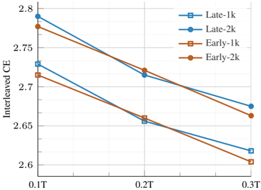
## Line Chart: Interleaved CE vs. T (Model Scale/Training Steps)
### Overview
The image displays a line chart plotting a metric called "Interleaved CE" against a variable "T" (likely representing model scale in trillions of parameters or training steps). The chart compares four different experimental configurations, showing a consistent downward trend for all series as T increases.
### Components/Axes
* **Chart Type:** Multi-series line chart with markers.
* **Y-Axis:**
* **Label:** "Interleaved CE" (likely Cross-Entropy loss).
* **Scale:** Linear, ranging from approximately 2.60 to 2.80.
* **Major Ticks:** 2.6, 2.65, 2.7, 2.75, 2.8.
* **X-Axis:**
* **Label:** Not explicitly labeled, but marked with values "0.1T", "0.2T", "0.3T". "T" likely denotes a unit of scale (e.g., Trillions of parameters) or training duration.
* **Scale:** Linear, with three discrete data points.
* **Legend:** Positioned in the top-right corner of the plot area. It defines four data series:
1. **Late-1k:** Blue line with hollow square markers (□).
2. **Late-2k:** Blue line with solid circle markers (●).
3. **Early-1k:** Orange line with hollow square markers (□).
4. **Early-2k:** Orange line with solid circle markers (●).
### Detailed Analysis
**Data Series and Approximate Values:**
The chart shows three data points for each series at x=0.1T, 0.2T, and 0.3T. Values are approximate based on visual interpolation against the y-axis grid.
1. **Late-1k (Blue, Hollow Square):**
* **Trend:** Steep downward slope.
* **Points:** (0.1T, ~2.78), (0.2T, ~2.655), (0.3T, ~2.62).
2. **Late-2k (Blue, Solid Circle):**
* **Trend:** Downward slope, less steep than Late-1k.
* **Points:** (0.1T, ~2.79), (0.2T, ~2.72), (0.3T, ~2.675).
3. **Early-1k (Orange, Hollow Square):**
* **Trend:** Steep downward slope, similar to Late-1k.
* **Points:** (0.1T, ~2.715), (0.2T, ~2.66), (0.3T, ~2.605).
4. **Early-2k (Orange, Solid Circle):**
* **Trend:** Downward slope, less steep than Early-1k.
* **Points:** (0.1T, ~2.775), (0.2T, ~2.72), (0.3T, ~2.665).
**Cross-Referenced Observations:**
* At **0.1T**, the "Late" configurations (blue lines) start at a higher Interleaved CE (~2.78-2.79) than the "Early" configurations (orange lines, ~2.715-2.775).
* At **0.3T**, the order changes. The "1k" variants (hollow squares) end at lower values (~2.605-2.62) than their "2k" counterparts (solid circles, ~2.665-2.675).
* The lines for **Late-2k** and **Early-2k** (solid circles) are nearly parallel and very close in value at 0.2T and 0.3T.
* The lines for **Late-1k** and **Early-1k** (hollow squares) also follow a similar, steeper trajectory.
### Key Observations
1. **Universal Improvement:** All four configurations show a decrease in Interleaved CE (improvement, assuming lower CE is better) as T increases from 0.1T to 0.3T.
2. **"1k" vs. "2k" Divergence:** The "1k" variants (hollow squares) exhibit a more significant rate of improvement (steeper slope) compared to the "2k" variants (solid circles). This suggests the "1k" setting benefits more from increased scale/T.
3. **"Late" vs. "Early" Convergence:** While "Late" starts worse (higher CE) than "Early" at 0.1T, the gap narrows considerably by 0.3T, especially for the "2k" variants where the lines nearly meet.
4. **Potential Crossover:** The **Late-1k** line appears to cross below the **Early-2k** line between 0.2T and 0.3T, indicating that with sufficient scale, the "Late-1k" configuration may outperform the "Early-2k" one.
### Interpretation
This chart likely visualizes results from an experiment in machine learning, comparing different training schedules ("Early" vs. "Late" intervention or data mixing) and context window sizes or sequence lengths ("1k" vs. "2k") across increasing model scales or training compute (T).
* **What the data suggests:** Increasing scale (T) universally reduces loss (Interleaved CE). However, the choice of schedule ("Early"/"Late") and sequence length ("1k"/"2k") significantly impacts both the starting performance and the rate of improvement.
* **Relationship between elements:** The "1k" configurations are more sensitive to scale, showing greater gains. The "Late" schedule starts at a disadvantage but catches up, suggesting it may be more effective at larger scales. The near-parallel lines for "2k" variants imply their relative performance is stable across the tested scale range.
* **Notable implication:** The most efficient configuration depends on the target scale. For smaller scale (0.1T), "Early-1k" is best. For larger scale (0.3T), "Late-1k" becomes the top performer. This highlights a potential trade-off between initial performance and scalability in model training design.