\n
## Chart: NMSE vs. Frequency for Different Methods
### Overview
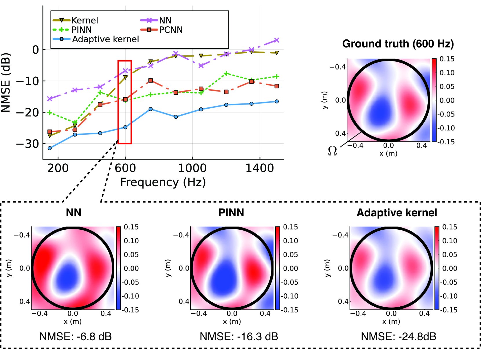
The image presents a chart comparing the Normalized Mean Squared Error (NMSE) in decibels (dB) across different frequencies (Hz) for four different methods: Kernel, Neural Network (NN), Physics-Informed Neural Network (PINN), and Probabilistic Convolutional Neural Network (PCNN). Below the main chart are visualizations of the ground truth and the results from each method at a specific frequency (600 Hz), represented as heatmaps.
### Components/Axes
* **X-axis:** Frequency (Hz), ranging from approximately 150 Hz to 1500 Hz. Marked at 200, 600, 1000, and 1400 Hz.
* **Y-axis:** NMSE (dB), ranging from approximately -30 dB to 0 dB. Marked at -30, -20, -10, 0, 10.
* **Legend:** Located in the top-left corner, identifying the data series:
* Kernel (Red, triangle markers)
* NN (Magenta, cross markers)
* PINN (Green, plus markers)
* PCNN (Blue, circle markers)
* **Ground Truth Heatmap:** Top-right corner, labeled "Ground truth (600 Hz)". X-axis labeled "x (m)", ranging from -0.15 to 0.4. Y-axis labeled "y (m)", ranging from -0.4 to 0.4.
* **Method Heatmaps:** Bottom row, labeled "NN", "PINN", and "Adaptive kernel" respectively. Each heatmap has the same x and y axis scales as the ground truth.
* **NMSE Values:** Below each method heatmap, the NMSE value in dB is displayed.
### Detailed Analysis or Content Details
**Main Chart (NMSE vs. Frequency):**
* **Kernel:** Starts at approximately -25 dB at 200 Hz, increases to around -10 dB at 600 Hz, then decreases to approximately -15 dB at 1400 Hz.
* **NN:** Starts at approximately 10 dB at 200 Hz, increases to around 15 dB at 600 Hz, then decreases to approximately 5 dB at 1400 Hz.
* **PINN:** Starts at approximately -20 dB at 200 Hz, increases to around -5 dB at 600 Hz, then remains relatively stable at around -10 dB at 1400 Hz.
* **PCNN:** Starts at approximately -5 dB at 200 Hz, remains relatively stable around -10 dB to -15 dB between 200 Hz and 1000 Hz, then increases to approximately -5 dB at 1400 Hz.
**Heatmaps (600 Hz):**
* **Ground Truth:** Shows a bipolar pattern with a positive lobe in the top-right and a negative lobe in the bottom-left. The color scale ranges from approximately -0.10 (dark red) to 0.15 (dark blue).
* **NN:** Similar bipolar pattern to the ground truth, but with less distinct lobes and a slightly shifted center. NMSE: -6.8 dB.
* **PINN:** Shows a more diffused pattern compared to the ground truth, with less clear separation between the positive and negative lobes. NMSE: -16.3 dB.
* **Adaptive Kernel:** Displays a pattern closest to the ground truth, with well-defined lobes and a similar shape. NMSE: -24.8 dB.
### Key Observations
* The Adaptive Kernel method consistently exhibits the lowest NMSE values across all frequencies, indicating the best performance.
* The NN method generally has the highest NMSE values, suggesting the poorest performance.
* The NMSE values for all methods tend to increase around 600 Hz, indicating a potential challenge in accurately modeling the system at that frequency.
* The heatmaps visually demonstrate the accuracy of each method in reproducing the ground truth pattern at 600 Hz. The Adaptive Kernel heatmap is the most similar to the ground truth.
### Interpretation
The data suggests that the Adaptive Kernel method is the most effective for modeling the system under investigation, as evidenced by its consistently low NMSE values. The NN method performs the worst, indicating that a simple neural network may not be sufficient to capture the underlying physics or complexity of the system. The PINN method shows moderate performance, potentially benefiting from the incorporation of physics-based information, but still falling short of the Adaptive Kernel.
The increase in NMSE around 600 Hz for all methods could indicate a resonance frequency or a region of increased sensitivity in the system. The heatmaps provide a visual representation of the errors, showing how each method deviates from the ground truth. The Adaptive Kernel's heatmap closely resembles the ground truth, confirming its superior performance.
The comparison of these methods highlights the importance of choosing an appropriate modeling technique based on the specific characteristics of the system being studied. The Adaptive Kernel's success suggests that a more sophisticated approach, potentially incorporating adaptive techniques, is crucial for achieving high accuracy.