## Chart/Diagram Type: Comparative Analysis of Acoustic Reconstruction Methods
### Overview
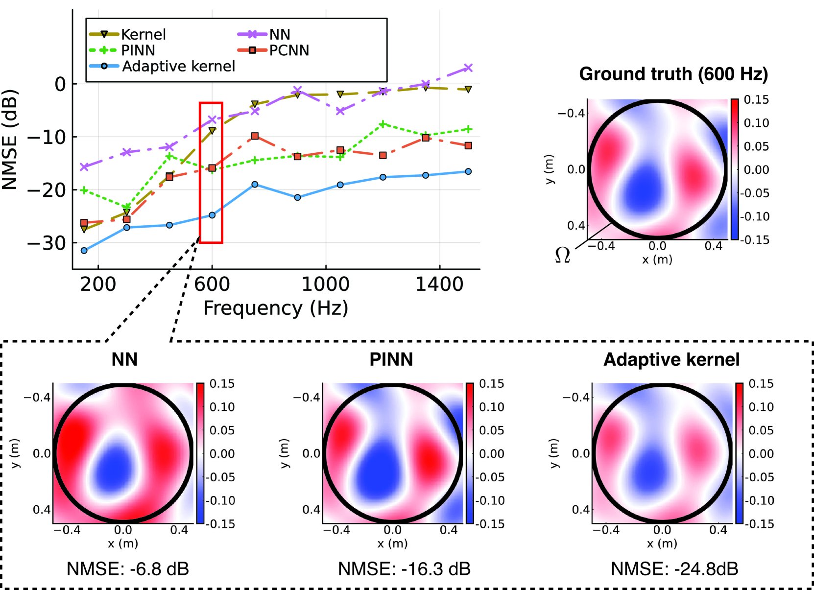
The image presents a comparative analysis of different methods for acoustic reconstruction, focusing on their performance in terms of Normalized Mean Square Error (NMSE) across a range of frequencies. It includes a line graph comparing the NMSE of Kernel, PINN, Adaptive kernel, NN, and PCNN methods, along with visualizations of the reconstructed acoustic fields for Ground Truth, NN, PINN, and Adaptive kernel at 600 Hz.
### Components/Axes
**1. Line Graph:**
* **X-axis:** Frequency (Hz), with markers at 200, 600, 1000, and 1400 Hz.
* **Y-axis:** NMSE (dB), ranging from -30 to 0 dB.
* **Legend (top-left):**
* Yellow-green line with downward-pointing triangles: Kernel
* Green dashed line with plus signs: PINN
* Blue line with circles: Adaptive kernel
* Purple line with crosses: NN
* Red line with squares: PCNN
**2. Acoustic Field Visualizations (right and bottom):**
* **Title (top-right):** Ground truth (600 Hz)
* **Titles (bottom):** NN, PINN, Adaptive kernel
* **Axes:**
* x-axis: x (m), ranging from -0.4 to 0.4
* y-axis: y (m), ranging from -0.4 to 0.4
* **Color scale:** Represents acoustic pressure, ranging from -0.15 (blue) to 0.15 (red).
* **NMSE values (below each visualization):**
* NN: -6.8 dB
* PINN: -16.3 dB
* Adaptive kernel: -24.8 dB
### Detailed Analysis or ### Content Details
**1. Line Graph Analysis:**
* **Kernel (Yellow-green triangles):** NMSE starts at approximately -27 dB at 200 Hz, rises to about -3 dB at 1400 Hz.
* **PINN (Green dashed line):** NMSE starts at approximately -20 dB at 200 Hz, dips to -23 dB at 400 Hz, then rises to approximately -7 dB at 1400 Hz.
* **Adaptive kernel (Blue circles):** NMSE starts at approximately -31 dB at 200 Hz, rises to approximately -18 dB at 1400 Hz.
* **NN (Purple crosses):** NMSE starts at approximately -13 dB at 200 Hz, rises to approximately -2 dB at 1400 Hz.
* **PCNN (Red squares):** NMSE starts at approximately -26 dB at 200 Hz, rises to approximately -12 dB at 1400 Hz.
**2. Acoustic Field Visualizations:**
* **Ground Truth (600 Hz):** Shows a characteristic pattern with two main lobes of opposite polarity (red and blue) within a circular region.
* **NN:** Reconstructed field shows a similar pattern to the ground truth, but with less distinct lobes.
* **PINN:** Reconstructed field shows a similar pattern to the ground truth, but with less distinct lobes.
* **Adaptive kernel:** Reconstructed field shows a pattern very similar to the ground truth, with well-defined lobes.
### Key Observations
* The Adaptive kernel method consistently exhibits the lowest NMSE across the frequency range, indicating superior performance in acoustic reconstruction.
* The NN method generally has the highest NMSE, suggesting it is the least accurate among the methods compared.
* The acoustic field visualizations at 600 Hz visually confirm the NMSE results, with the Adaptive kernel reconstruction appearing closest to the ground truth.
* The performance of all methods generally degrades (NMSE increases) as frequency increases.
### Interpretation
The data suggests that the Adaptive kernel method is the most effective for acoustic reconstruction in this scenario, as it minimizes the error between the reconstructed and actual acoustic fields. The NN method, on the other hand, appears to be the least effective. The visualizations provide a qualitative assessment that supports the quantitative NMSE results. The increase in NMSE with frequency indicates that all methods face challenges in accurately reconstructing acoustic fields at higher frequencies. The choice of method would depend on the specific application and the trade-off between computational complexity and accuracy.