## Mathematical Plot Pair: Energy Dispersion Relations
### Overview
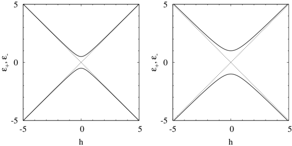
The image displays two side-by-side, square-format mathematical plots. Each plot shows two curves (one solid, one dashed) on a 2D Cartesian coordinate system. The plots appear to represent energy dispersion relations or eigenvalue solutions as a function of a parameter `h`. The left plot exhibits an "avoided crossing" behavior, while the right plot shows a direct crossing of the two curves.
### Components/Axes
**Common to Both Plots:**
* **Y-axis:** Labeled with the Greek letters `ε₊` (epsilon plus) and `ε₋` (epsilon minus). The axis scale ranges from -5 to 5, with major tick marks at -5, 0, and 5.
* **X-axis:** Labeled with the letter `h`. The axis scale ranges from -5 to 5, with major tick marks at -5, 0, and 5.
* **Data Series:** Each plot contains two data series differentiated by line style:
1. A **solid black line**.
2. A **dashed black line**.
* **Plot Frame:** Each graph is enclosed in a square box with tick marks on all four sides.
**Spatial Layout:**
* The two plots are arranged horizontally, side-by-side.
* The y-axis labels (`ε₊, ε₋`) are positioned to the left of each plot's vertical axis.
* The x-axis label (`h`) is centered below each plot's horizontal axis.
### Detailed Analysis
**Left Plot Analysis:**
* **Trend Verification:** Both curves are symmetric about the vertical line `h=0`. As `|h|` increases (moving left or right from the center), both curves move away from the horizontal axis (`ε=0`) in opposite directions. The solid line trends upward, and the dashed line trends downward.
* **Key Feature:** The curves approach each other near `h=0` but do not intersect. They reach a point of closest approach (a minimum gap) at `h=0`. At this point, the solid line is at a positive `ε` value (approximately `ε ≈ 0.8`), and the dashed line is at a negative `ε` value (approximately `ε ≈ -0.8`).
* **Behavior at Extremes:** At `h = -5` and `h = 5`, the solid line reaches `ε ≈ 5`, and the dashed line reaches `ε ≈ -5`.
**Right Plot Analysis:**
* **Trend Verification:** Both curves are also symmetric about `h=0`. As `|h|` increases, both curves move away from `ε=0` in opposite directions, similar to the left plot.
* **Key Feature:** The two curves intersect directly at the origin point `(h=0, ε=0)`. This is a crossing point, not an avoided crossing.
* **Behavior at Extremes:** At `h = -5` and `h = 5`, the solid line reaches `ε ≈ 5`, and the dashed line reaches `ε ≈ -5`, identical to the left plot.
### Key Observations
1. **Symmetry:** Both plots exhibit perfect symmetry about the `h=0` axis.
2. **Line Style Consistency:** The solid line represents the upper branch (positive `ε`) for `h>0` and the lower branch (negative `ε`) for `h<0` in both plots. The dashed line does the opposite.
3. **Critical Difference:** The fundamental distinction between the two plots is the behavior at `h=0`. The left plot shows a **finite energy gap** (avoided crossing), while the right plot shows a **zero energy gap** (crossing).
4. **Identical Asymptotes:** Far from `h=0` (at `|h| = 5`), the numerical values of the curves are identical in both plots, suggesting the same underlying linear relationship dominates at large `|h|`.
### Interpretation
These plots are characteristic of a two-level quantum system or a coupled oscillator model, where `ε` represents energy or frequency and `h` represents a tuning parameter like a magnetic field or detuning.
* **Left Plot (Avoided Crossing):** This demonstrates the effect of a **coupling** or interaction between the two states. The interaction prevents the energy levels from crossing, creating a minimum gap at the resonance point (`h=0`). This is a signature of hybridization, where the original states mix to form new eigenstates with separated energies. The size of the gap at `h=0` is proportional to the coupling strength.
* **Right Plot (Crossing):** This represents the **uncoupled** or degenerate case. The two states are independent, and their energies cross linearly as the parameter `h` is varied. There is no interaction to lift the degeneracy at the crossing point.
* **Relationship:** The pair of plots likely illustrates a comparison between a system with interaction (left) and without interaction (right). The identical behavior at large `|h|` indicates that the coupling is a local effect near resonance (`h=0`), while the far-detuned behavior is governed by the bare, uncoupled energies.
* **Underlying Model:** The linear dependence of `ε` on `h` at large `|h|` suggests a Hamiltonian of the form `H ~ hσ_z` (where `σ_z` is a Pauli matrix), with an additional coupling term `~ σ_x` present only in the left plot. The avoided crossing gap is `2 * |coupling strength|`.