## [Chart/Diagram Type]: Comparative Analysis of $V_{\phi^4}$ and $V_{XY}$ Models
### Overview
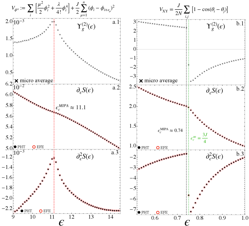
The image presents a comparative analysis of two physical models, $V_{\phi^4}$ (left column) and $V_{XY}$ (right column), across three different metrics (rows). Each column displays three vertically stacked plots showing the behavior of specific functions ($Y_g^{(2)}$, $\partial_\epsilon S$, and $\partial_\epsilon^2 S$) relative to a parameter $\epsilon$. The plots illustrate critical phenomena, likely phase transitions, with specific critical values ($\epsilon_c$) highlighted by vertical lines.
### Components/Axes
**Top Formulas:**
* **Left:** $V_{\phi^4} := \sum_i [\frac{\mu^2}{2}\phi_i^2 + \frac{\lambda}{4!}\phi_i^4] + \frac{J}{2}\sum_{\mu=1}^n (\phi_i - \phi_{i+e_\mu})^2$
* **Right:** $V_{XY} = \frac{J}{2N} \sum_{i,j} [1 - \cos(\theta_i - \theta_j)]$
**Plot Structure:**
* **Left Column (a.1, a.2, a.3):** X-axis represents $\epsilon$ ranging from 9 to 14.
* **Right Column (b.1, b.2, b.3):** X-axis represents $\epsilon$ ranging from 0.55 to 1.0.
* **Legends:**
* **a.1/b.1:** "x micro average" (represented by black 'x' markers).
* **a.2/a.3/b.2/b.3:** "PHT" (black filled circle) and "EFE" (red open circle).
* **Annotations:**
* **a.2:** $\epsilon_c^{MIPA} \approx 11.1$ (indicated by a red dashed vertical line).
* **b.2:** $\epsilon_c^{MIPA} \approx 0.74$ (indicated by a black dashed vertical line) and $\epsilon_c^\infty = \frac{3J}{4}$ (indicated by a green dashed vertical line).
### Detailed Analysis
#### Left Column: $V_{\phi^4}$
* **a.1 ($Y_g^{(2)}(\epsilon)$):**
* **Trend:** The data points (black 'x') form a sharp peak. The values increase from $\approx 1.4 \times 10^{-3}$ at $\epsilon=9$ to a maximum of $\approx 2.0 \times 10^{-3}$ at $\epsilon \approx 11.1$, then decrease sharply to $\approx 0.2 \times 10^{-3}$ at $\epsilon=14.5$.
* **a.2 ($\partial_\epsilon S(\epsilon)$):**
* **Trend:** The data (PHT/EFE) shows a smooth, monotonically decreasing curve.
* **Values:** Starts at $\approx 6.05 \times 10^{-2}$ at $\epsilon=9$ and decreases to $\approx 5.0 \times 10^{-2}$ at $\epsilon=14.5$.
* **Note:** The PHT and EFE data points are perfectly superimposed.
* **a.3 ($\partial_\epsilon^2 S(\epsilon)$):**
* **Trend:** The data (PHT/EFE) shows a sharp cusp/peak at $\epsilon \approx 11.1$.
* **Values:** Increases from $\approx -2.2 \times 10^{-3}$ at $\epsilon=9$ to a peak of $\approx -1.2 \times 10^{-3}$ at $\epsilon \approx 11.1$, then decreases back to $\approx -2.2 \times 10^{-3}$ at $\epsilon=14.5$.
#### Right Column: $V_{XY}$
* **b.1 ($Y_g^{(2)}(\epsilon)$):**
* **Trend:** The data (black 'x') shows a discontinuity at $\epsilon \approx 0.74$.
* **Values:** Decreases from $\approx 3.0$ at $\epsilon=0.55$ to $\approx 2.5$ at $\epsilon \approx 0.74$. Immediately after the discontinuity, the value drops to $\approx -3.5$ and then increases towards $\approx -1.0$ at $\epsilon=1.0$.
* **b.2 ($\partial_\epsilon S(\epsilon)$):**
* **Trend:** The data (PHT/EFE) shows a discontinuity at $\epsilon \approx 0.74$.
* **Values:** Decreases from $\approx 2.5$ at $\epsilon=0.55$ to $\approx 2.0$ at $\epsilon \approx 0.74$. After the discontinuity, it drops to $\approx 1.5$ and continues to decrease to $\approx 1.0$ at $\epsilon=1.0$.
* **b.3 ($\partial_\epsilon^2 S(\epsilon)$):**
* **Trend:** The data (PHT/EFE) shows a sharp discontinuity at $\epsilon \approx 0.74$.
* **Values:** Increases from $\approx -3.2$ at $\epsilon=0.55$ to $\approx -1.5$ at $\epsilon \approx 0.74$. After the discontinuity, it drops sharply to $\approx -6.5$ and then increases towards $\approx -2.0$ at $\epsilon=1.0$.
### Key Observations
* **Data Superposition:** In all plots containing both PHT and EFE markers (a.2, a.3, b.2, b.3), the red open circles (EFE) and black filled circles (PHT) are perfectly aligned, indicating identical results from both methods.
* **Critical Behavior:** The vertical lines denote critical values ($\epsilon_c$).
* The left column ($V_{\phi^4}$) exhibits continuous behavior with a peak/cusp at $\epsilon_c$.
* The right column ($V_{XY}$) exhibits a clear discontinuity (jump) at $\epsilon_c$, characteristic of a first-order phase transition.
* **Consistency:** The "micro average" data points (black 'x') are consistent with the trends observed in the PHT/EFE data series.
### Interpretation
The data demonstrates the behavior of two distinct physical systems near critical points.
* **$V_{\phi^4}$ (Left):** The continuous nature of the derivatives suggests a second-order (continuous) phase transition. The peak in $Y_g^{(2)}$ and the cusp in $\partial_\epsilon^2 S$ at $\epsilon \approx 11.1$ are hallmarks of critical fluctuations.
* **$V_{XY}$ (Right):** The sharp discontinuities in all three metrics at $\epsilon \approx 0.74$ strongly suggest a first-order (discontinuous) phase transition. The system undergoes a sudden change in state at this critical value.
* **Methodology:** The perfect overlap between PHT (likely Perturbative Hartree) and EFE (likely Effective Field Theory/Equation) suggests that both theoretical frameworks are in excellent agreement for these specific models. The inclusion of $\epsilon_c^\infty = \frac{3J}{4}$ in plot b.2 provides an analytical reference point for the observed numerical discontinuity.