## Multi-Panel Scientific Figure: Critical Behavior Analysis
### Overview
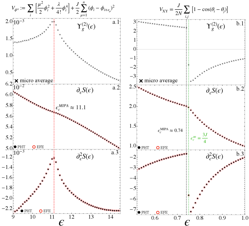
The image is a composite scientific figure containing two mathematical equations at the top and six plots arranged in a 3x2 grid below. The left column (labeled a.1, a.2, a.3) and the right column (labeled b.1, b.2, b.3) present related analyses for two different systems or parameter regimes. The plots show the behavior of various functions with respect to a parameter ε (epsilon). Key features include vertical dashed lines indicating critical points and annotations for specific values.
### Components/Axes
**Equations (Top):**
1. **Left Equation:** `V_φψ := Σ_i [ (μ²/2)φ_i² + (λ/4!)φ_i⁴ ] + (J/2) Σ_{μ=1}^n (φ_i - φ_{i+e_μ})²`
2. **Right Equation:** `V_XY = (J/2N) Σ_{i,j} [1 - cos(θ_i - θ_j)]`
**Plot Grid Structure:**
* **X-axis (All plots):** Labeled `ε` (epsilon).
* **Column a (Left):** Range approximately 9 to 14.5.
* **Column b (Right):** Range approximately 0.55 to 1.0.
* **Y-axes (By Row):**
* **Row 1 (a.1, b.1):** Labeled `γ_g^(2)(ε)`. Scale is linear.
* **Row 2 (a.2, b.2):** Labeled `∂_ε S(ε)`. Scale is linear.
* **Row 3 (a.3, b.3):** Labeled `∂_ε^2 S(ε)`. Scale is linear.
* **Legends & Annotations:**
* **"micro average"**: Marked with a black 'x' symbol in plots a.1 and b.1.
* **"PHT"**: Represented by a solid black circle (●). Appears in the legend of plots a.2, a.3, b.2, b.3.
* **"EFE"**: Represented by a red open circle (○). Appears in the legend of plots a.2, a.3, b.2, b.3.
* **Vertical Dashed Lines:**
* **Column a:** A red vertical dashed line at `ε ≈ 11.1`. Annotated in plot a.2 as `ε_c^MIPA ≈ 11.1`.
* **Column b:** A green vertical dashed line at `ε ≈ 0.74`. Annotated in plot b.2 as `ε_c^MIPA ≈ 0.74`. An additional green text annotation in plot b.2 states `ε_c^∞ = 3J/4`.
* **Data Series:** Plots in rows 2 and 3 contain two data series: black dots (presumably for "PHT") and red circles (presumably for "EFE").
### Detailed Analysis
**Column a (Left Side):**
* **a.1 (`γ_g^(2)(ε)`):** The curve (gray 'x' markers) shows a sharp peak at the critical point `ε ≈ 11.1`. The value rises from ~1.4x10⁻³ at ε=9 to a peak of ~2.0x10⁻³, then decays.
* **a.2 (`∂_ε S(ε)`):** Both data series (black dots/PHT and red circles/EFE) show a nearly linear, decreasing trend. The values drop from ~6.2x10⁻² at ε=9 to ~5.0x10⁻² at ε=14.5. The two series are nearly indistinguishable. The critical point `ε_c^MIPA ≈ 11.1` is marked.
* **a.3 (`∂_ε^2 S(ε)`):** The data shows a pronounced, sharp peak (a cusp) at the critical point `ε ≈ 11.1`. The value rises from ~-2.2x10⁻³ at ε=9 to a peak of ~-1.2x10⁻³, then decays back down. The black (PHT) and red (EFE) series overlap closely.
**Column b (Right Side):**
* **b.1 (`γ_g^(2)(ε)`):** The curve (gray 'x' markers) shows a discontinuity or very sharp change at the critical point `ε ≈ 0.74`. The value is high (~2.8) for ε < 0.74, drops abruptly, and then increases from ~-3.5 to ~-1.0 for ε > 0.74.
* **b.2 (`∂_ε S(ε)`):** Both data series show a decreasing trend. The values drop from ~2.5 at ε=0.55 to ~1.0 at ε=1.0. The slope appears to change near the critical point `ε_c^MIPA ≈ 0.74`. The annotation `ε_c^∞ = 3J/4` is present.
* **b.3 (`∂_ε^2 S(ε)`):** The data shows a sharp, downward cusp (a minimum) at the critical point `ε ≈ 0.74`. The value falls from ~-3.0 at ε=0.55 to a minimum of ~-7.0, then rises back to ~-2.0 at ε=1.0. The black (PHT) and red (EFE) series overlap closely.
### Key Observations
1. **Critical Points:** Both systems exhibit critical behavior at specific ε values (`~11.1` for column a, `~0.74` for column b), marked by vertical lines and singularities in the plotted functions.
2. **Nature of Singularity:** The singularity manifests differently. In column a, `γ_g^(2)` shows a peak and `∂_ε^2 S` shows a cusp. In column b, `γ_g^(2)` shows a discontinuity and `∂_ε^2 S` shows a sharp minimum.
3. **Data Series Agreement:** The "PHT" (black dots) and "EFE" (red circles) data series are in very close agreement across all plots where they appear (rows 2 and 3), suggesting two different methods or approximations yield nearly identical results for these quantities.
4. **Equation Context:** The equations at the top define potentials (`V_φψ` and `V_XY`) for what appear to be field theories (possibly φ⁴ theory and an XY model), providing the theoretical context for the analyzed data.
### Interpretation
This figure presents a comparative analysis of critical phenomena in two different statistical mechanical or field-theoretic models. The left column (a) likely corresponds to a system with a continuous (second-order) phase transition, evidenced by the continuous but non-differentiable cusp in the second derivative of entropy (`∂_ε^2 S`). The right column (b) suggests a system with a more abrupt transition, possibly first-order or of a different universality class, indicated by the apparent discontinuity in `γ_g^(2)`.
The parameter ε is the control parameter driving the system through its critical point (`ε_c`). The functions plotted—`γ_g^(2)` (likely a correlation function or susceptibility), the first derivative of entropy `∂_ε S` (related to specific heat or a response function), and its second derivative `∂_ε^2 S`—are standard quantities for characterizing phase transitions. The sharp features at `ε_c` are hallmarks of critical behavior, where correlation lengths diverge and the system becomes scale-invariant.
The close match between "PHT" and "EFE" data suggests the figure is validating a theoretical or computational method (perhaps "EFE" stands for an Effective Field Theory approach) against another standard ("PHT"). The annotation `ε_c^∞ = 3J/4` in plot b.2 provides an analytical prediction for the critical point in a certain limit (∞), which the numerical/data-driven `ε_c^MIPA ≈ 0.74` approximates. The overall purpose is to demonstrate and quantify the critical behavior of these models, locate their critical points, and compare different calculational approaches.