## Chart/Diagram Type: Dual-Axis Graphs with Subplots
### Overview
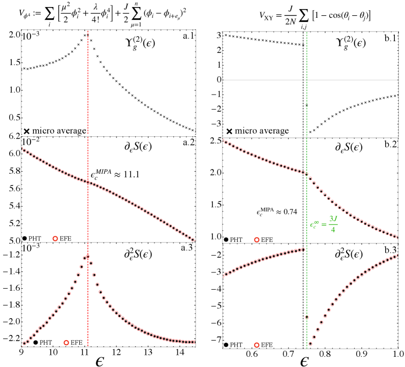
The image contains two side-by-side graphs (labeled **a** and **b**), each divided into three subplots (a.1, a.2, a.3 and b.1, b.2, b.3). These graphs depict mathematical functions and their derivatives as functions of a parameter **ε** (epsilon). Key elements include legends, vertical dashed lines, and annotations for critical points.
---
### Components/Axes
#### Left Graph (a):
- **a.1**:
- **X-axis**: **ε** (epsilon), ranging from 9 to 14.
- **Y-axis**: **V_φ4** (top plot), **Γ_g^(2)(ε)** (middle plot), **δ_εS(ε)** (bottom plot).
- **Legend**:
- **PHT**: Black dots (bottom-left corner).
- **EFE**: Red circles (bottom-left corner).
- **Annotations**:
- Vertical red dashed line at **ε_c^MIPA ≈ 11.1**.
- Micro average marked with a cross (x) at **ε ≈ 10.5**.
- **a.2**:
- **X-axis**: **ε** (epsilon), same range as a.1.
- **Y-axis**: **δ_εS(ε)** (top plot), **δ²_εS(ε)** (bottom plot).
- **a.3**:
- **X-axis**: **ε** (epsilon), same range as a.1.
- **Y-axis**: **δ²_εS(ε)** (bottom plot).
#### Right Graph (b):
- **b.1**:
- **X-axis**: **ε** (epsilon), ranging from 0.6 to 1.0.
- **Y-axis**: **V_XY** (top plot), **Γ_g^(2)(ε)** (middle plot).
- **Legend**:
- **PHT**: Black dots (bottom-left corner).
- **EFE**: Red circles (bottom-left corner).
- **Annotations**:
- Vertical green dashed line at **ε_c^∞ = 3J/4**.
- Micro average marked with a cross (x) at **ε ≈ 0.75**.
- **b.2**:
- **X-axis**: **ε** (epsilon), same range as b.1.
- **Y-axis**: **δ_εS(ε)** (top plot), **δ²_εS(ε)** (bottom plot).
- **b.3**:
- **X-axis**: **ε** (epsilon), same range as b.1.
- **Y-axis**: **δ²_εS(ε)** (bottom plot).
---
### Detailed Analysis
#### Left Graph (a):
1. **a.1**:
- **V_φ4**: Peaks near **ε ≈ 10.5**, then declines.
- **Γ_g^(2)(ε)**: Dips sharply at **ε ≈ 10.5**, then rises.
- **δ_εS(ε)**: Decreases monotonically from **ε = 9** to **ε = 14**.
- **δ²_εS(ε)**: Shows a sharp minimum at **ε ≈ 10.5**, with values dropping to **-2.2**.
2. **a.2**:
- **δ_εS(ε)**: Decreases from **6.0** at **ε = 9** to **5.0** at **ε = 14**.
- **δ²_εS(ε)**: Peaks at **ε ≈ 10.5** (value ~-1.6), then declines.
3. **a.3**:
- **δ²_εS(ε)**: Minimum at **ε ≈ 10.5** (value ~-2.2), with a secondary minimum at **ε ≈ 14**.
#### Right Graph (b):
1. **b.1**:
- **V_XY**: Peaks at **ε ≈ 0.7**, then declines.
- **Γ_g^(2)(ε)**: Rises sharply at **ε ≈ 0.7**, then plateaus.
- **δ_εS(ε)**: Decreases from **2.5** at **ε = 0.6** to **1.0** at **ε = 1.0**.
- **δ²_εS(ε)**: Peaks at **ε ≈ 0.7** (value ~-5), then declines.
2. **b.2**:
- **δ_εS(ε)**: Decreases from **2.5** at **ε = 0.6** to **1.0** at **ε = 1.0**.
- **δ²_εS(ε)**: Peaks at **ε ≈ 0.7** (value ~-5), then declines.
3. **b.3**:
- **δ²_εS(ε)**: Minimum at **ε ≈ 0.7** (value ~-5), with a secondary minimum at **ε ≈ 1.0**.
---
### Key Observations
1. **Critical Points**:
- Left graph: **ε_c^MIPA ≈ 11.1** (red dashed line) marks a phase transition or critical threshold.
- Right graph: **ε_c^∞ = 3J/4** (green dashed line) indicates a theoretical limit.
2. **Micro Averages**:
- Crosses (x) in both graphs highlight averaged values at **ε ≈ 10.5** (left) and **ε ≈ 0.75** (right).
3. **Function Behavior**:
- **V_φ4** and **V_XY** exhibit peaks near their respective critical points.
- **δ²_εS(ε)** in both graphs shows minima at critical points, suggesting stability or optimal conditions.
4. **Legend Consistency**:
- **PHT** (black dots) and **EFE** (red circles) are consistently placed in the bottom-left corner of all subplots.
---
### Interpretation
The graphs likely represent a physical or mathematical model where **ε** governs system behavior. The critical points (**ε_c^MIPA** and **ε_c^∞**) demarcate distinct regimes:
- **Left Graph (a)**: Dominated by **V_φ4** and **Γ_g^(2)(ε)**, with **δ²_εS(ε)** minima indicating stability at **ε ≈ 10.5**.
- **Right Graph (b)**: Governed by **V_XY** and **Γ_g^(2)(ε)**, with **δ²_εS(ε)** minima at **ε ≈ 0.7**, suggesting a phase transition or optimal parameter range.
The equations embedded in the plots (e.g., **V_φ4 = Σ[μ²φ_i²/2 + λ/4!φ_i⁴] + J/2 Σ(φ_i - φ_{i+ε})²**) imply interactions between variables, possibly in a lattice or network model. The **PHT** and **EFE** markers may represent different experimental or theoretical datasets, with **EFE** showing sharper transitions near critical points.
The **δ²_εS(ε)** minima in both graphs highlight regions of minimal variance, critical for understanding system stability or phase behavior. The **micro averages** (crosses) suggest averaged trends over a range of **ε**, contrasting with the detailed data points (dots and circles).
This analysis underscores the interplay between **ε**, critical thresholds, and system stability, with potential applications in statistical mechanics, material science, or complex systems theory.