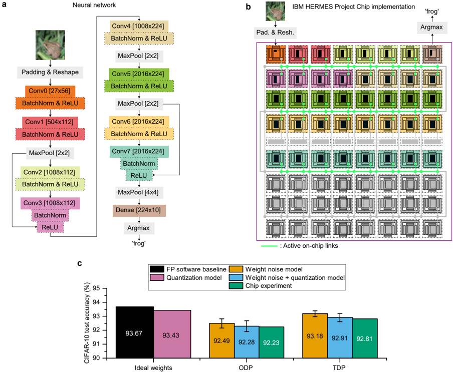
## Neural Network and Chip Implementation Diagram with Performance Chart ### Overview The image presents a neural network architecture, its chip implementation, and a performance comparison chart. Part (a) illustrates the neural network structure, part (b) shows the chip implementation of the network, and part (c) compares the CIFAR-10 test accuracy of different models (FP software baseline, quantization model, weight noise model, weight noise + quantization model, and chip experiment) under different conditions (Ideal weights, ODP, TDP). ### Components/Axes **Part (a): Neural Network** * **Title:** Neural network * **Input:** Image of a frog * **Layers:** * Padding & Reshape * Conv0 [27x56] + BatchNorm & ReLU * Conv1 [504x112] + BatchNorm & ReLU * MaxPool [2x2] * Conv2 [1008x112] + BatchNorm & ReLU * Conv3 [1008x112] + BatchNorm & ReLU * Conv4 [1008x224] + BatchNorm & ReLU * MaxPool [2x2] * Conv5 [2016x224] + BatchNorm & ReLU * MaxPool [2x2] * Conv6 [2016x224] + BatchNorm & ReLU * Conv7 [2016x224] + BatchNorm & ReLU * MaxPool [4x4] * Dense [224x10] * Argmax * **Output:** 'frog' **Part (b): IBM HERMES Project Chip Implementation** * **Title:** IBM HERMES Project Chip implementation * **Input:** Image of a frog, Pad. & Resh. * **Output:** Argmax -> 'frog' * **Chip Structure:** A grid of processing units, with different units highlighted in colors corresponding to the layers in part (a). * **Active on-chip links:** Indicated by green lines connecting the processing units. * The entire chip is enclosed in a purple box. **Part (c): CIFAR-10 Test Accuracy Chart** * **Title:** CIFAR-10 test accuracy (%) * **Y-axis:** CIFAR-10 test accuracy (%), ranging from 90 to 95. * **X-axis:** Categorical labels: Ideal weights, ODP, TDP. * **Legend (located in the top-right):** * Black: FP software baseline * Pink: Quantization model * Orange: Weight noise model * Purple: Weight noise + quantization model * Teal: Chip experiment ### Detailed Analysis or ### Content Details **Part (a): Neural Network** The neural network consists of convolutional layers (Conv), batch normalization (BatchNorm), ReLU activation functions, max pooling layers (MaxPool), and a dense layer. The input image undergoes padding and reshaping before being processed by the convolutional layers. The dimensions of each layer are indicated in brackets (e.g., Conv0 [27x56]). **Part (b): IBM HERMES Project Chip Implementation** The chip implementation shows a grid of processing units, with connections between them. The colors of the units correspond to the layers in the neural network architecture. The green lines indicate active on-chip links. **Part (c): CIFAR-10 Test Accuracy Chart** The chart compares the performance of different models on the CIFAR-10 dataset. * **Ideal weights:** * FP software baseline (Black): 93.67% * Quantization model (Pink): 93.43% * **ODP:** * Weight noise model (Orange): 92.49% +/- 0.2% * Weight noise + quantization model (Purple): 92.28% +/- 0.2% * Chip experiment (Teal): 92.23% +/- 0.2% * **TDP:** * Weight noise model (Orange): 93.18% +/- 0.2% * Weight noise + quantization model (Purple): 92.91% +/- 0.2% * Chip experiment (Teal): 92.81% +/- 0.2% ### Key Observations * The FP software baseline and quantization model achieve the highest accuracy with ideal weights. * The accuracy decreases when weight noise is introduced (ODP and TDP). * The chip experiment performance is comparable to the weight noise and quantization models. * The error bars on the ODP and TDP groups are small, indicating low variance. ### Interpretation The data suggests that the chip implementation achieves comparable performance to software models with weight noise and quantization. The ideal weight models (FP software baseline and quantization model) perform better, indicating that the chip implementation introduces some level of noise or approximation. The chart demonstrates the impact of weight noise and quantization on the accuracy of the neural network and provides a comparison of the chip implementation's performance against these models. The neural network diagram shows the flow of data and the transformations applied to the input image. The chip implementation diagram shows how the neural network is mapped onto the hardware.

## Diagram & Chart Compilation: Neural Network Architecture, Chip Implementation, and Accuracy Comparison ### Overview The image presents a compilation of three distinct but related elements: (a) a diagram illustrating the architecture of a neural network, (b) a visual representation of the IBM HERMES Project Chip implementation, and (c) a bar chart comparing the CIFAR-10 test accuracy of different models and implementations. The overall theme appears to be the implementation of a neural network on specialized hardware and the evaluation of its performance. ### Components/Axes **(a) Neural Network Diagram:** * **Components:** Padding & Reshape, Conv0, Conv1, Conv2, Conv3, Conv4, Conv5, Conv6, Conv7, Dense, Argmax. * **Layers & Dimensions:** Conv0 [27x56], Conv1 [504x112], Conv2 [1008x112], Conv3 [1008x112], Conv4 [1008x224], Conv5 [2016x224], Conv6 [2016x224], Conv7 [2016x224], Dense [224x10]. * **Operations:** BatchNorm & ReLU, MaxPool [2x2], MaxPool [4x4]. **(b) IBM HERMES Chip Implementation:** * **Labels:** "Pad. & Resh.", "Argmax", "frog", "Active on-chip links". * **Visual Representation:** A grid of colored squares representing the chip's structure, with connections indicated by lines. **(c) CIFAR-10 Test Accuracy Chart:** * **X-axis:** "Ideal weights", "ODP", "TDP". * **Y-axis:** "CIFAR-10 test accuracy (%)", ranging from 90 to 95. * **Legend:** * FP software baseline (Dark Red) * Quantization model (Purple) * Weight noise model (Blue) * Weight noise + quantization model (Green) * Chip experiment (Orange) ### Detailed Analysis or Content Details **(a) Neural Network Diagram:** The diagram shows a sequential flow of operations. The network begins with a Padding & Reshape layer, followed by a series of convolutional layers (Conv0 to Conv7) interspersed with Batch Normalization & ReLU activation functions and Max Pooling layers. The final layers consist of a Dense layer and an Argmax layer, which outputs "frog". The dimensions of each convolutional layer are explicitly stated. **(b) IBM HERMES Chip Implementation:** This section visually depicts the chip's architecture. The colored squares likely represent different processing units or memory blocks. The lines connecting these squares indicate data flow or communication pathways. The labels "Pad. & Resh." and "Argmax" suggest that these specific neural network operations are implemented within the chip. The image of a "frog" is present, likely related to the network's classification task. **(c) CIFAR-10 Test Accuracy Chart:** * **FP software baseline:** Approximately 93.67% accuracy across all three conditions (Ideal weights, ODP, TDP). * **Quantization model:** Approximately 93.43% accuracy across all three conditions. * **Weight noise model:** * Ideal weights: ~92.49% * ODP: ~92.28% * TDP: ~92.23% * **Weight noise + quantization model:** * Ideal weights: ~93.18% * ODP: ~92.91% * TDP: ~92.81% * **Chip experiment:** * Ideal weights: ~93.18% * ODP: ~92.91% * TDP: ~92.81% The error bars are present for the Weight noise model, Weight noise + quantization model, and Chip experiment. ### Key Observations * The FP software baseline consistently achieves the highest accuracy. * The quantization model shows a slight decrease in accuracy compared to the baseline. * Introducing weight noise further reduces accuracy, especially in the ODP and TDP conditions. * Combining weight noise and quantization results in accuracy levels similar to the weight noise model alone. * The chip experiment performs similarly to the weight noise + quantization model. * Accuracy tends to decrease slightly when moving from Ideal weights to ODP and TDP conditions for the models incorporating noise. ### Interpretation The data suggests that while the IBM HERMES chip can successfully implement the neural network, it introduces some performance degradation compared to a purely software-based implementation. The accuracy loss is likely due to the quantization and the introduction of noise during the chip's operation. The consistent performance of the chip experiment with the weight noise + quantization model indicates that the chip's limitations are closely tied to the effects of quantization and noise. The decreasing accuracy from Ideal weights to ODP and TDP suggests that these conditions represent increasing levels of hardware constraints or imperfections. ODP and TDP likely refer to different operating conditions or power/performance trade-offs within the chip. The presence of the "frog" label in both the neural network diagram and the chip implementation suggests that the network is designed for image classification, specifically identifying frogs. The overall study appears to be an evaluation of the trade-offs between accuracy, efficiency, and hardware constraints in deploying a neural network on a specialized chip. The data highlights the challenges of maintaining accuracy when moving from a software baseline to a hardware implementation, particularly when dealing with quantization and noise.

## Neural Network Architecture and Hardware Implementation Diagram ### Overview The image is a composite technical figure divided into three labeled panels (a, b, c). It illustrates the architecture of a convolutional neural network (CNN), its implementation on a specialized neuromorphic chip (IBM HERMES Project), and a performance comparison of different model variants on the CIFAR-10 dataset. The overall theme is the mapping of a deep learning model from a software definition to a physical hardware implementation and the evaluation of its accuracy under various non-ideal conditions. ### Components/Axes **Panel a: Neural Network Architecture** * **Input:** An image of a frog. * **Layers (in order of data flow):** 1. Padding & Reshape 2. Conv0 [27x56] → BatchNorm & ReLU 3. Conv1 [504x112] → BatchNorm & ReLU 4. MaxPool [2x2] 5. Conv2 [1008x112] → BatchNorm & ReLU 6. Conv3 [1008x112] → BatchNorm & ReLU 7. Conv4 [1008x224] → BatchNorm & ReLU 8. MaxPool [2x2] 9. Conv5 [2016x224] → BatchNorm & ReLU 10. MaxPool [2x2] 11. Conv6 [2016x224] → BatchNorm & ReLU 12. Conv7 [2016x224] → BatchNorm & ReLU 13. MaxPool [4x4] 14. Dense [224x10] 15. Argmax * **Output:** The classification label 'frog'. * **Note:** The diagram shows a sequential flow with some skip connections implied by the layout (e.g., Conv3 output feeds forward to Conv4). **Panel b: IBM HERMES Project Chip Implementation** * **Title:** "IBM HERMES Project Chip implementation" * **Input:** The same frog image, processed through "Pad. & Resh." (Padding & Reshape). * **Core Component:** A large grid representing the chip's core, composed of multiple processing elements (PEs) arranged in rows and columns. Each PE is depicted as a square with internal circuitry. * **Data Flow:** Green lines labeled "Active on-chip links" show the path of data through the grid of PEs, moving generally from top-left to bottom-right. * **Output:** The final processing element performs an "Argmax" operation, outputting the label 'frog'. * **Spatial Layout:** The chip grid is the central, dominant element. The input and output blocks are positioned at the top-left and top-right corners, respectively, outside the main grid. **Panel c: CIFAR-10 Test Accuracy Bar Chart** * **Chart Type:** Grouped bar chart with error bars. * **Y-Axis:** Label: "CIFAR-10 test accuracy (%)". Scale: 90 to 95, with major ticks at 90, 91, 92, 93, 94, 95. * **X-Axis Categories:** Three groups: "Ideal weights", "ODP", "TDP". * **Legend (Top Center):** Maps colors to model types: * Black: "FP software baseline" * Pink: "Quantization model" * Orange: "Weight noise model" * Blue: "Weight noise + quantization model" * Green: "Chip experiment" * **Data Series & Approximate Values (with error bars where visible):** * **Ideal weights:** * FP software baseline (Black): ~93.67% * Quantization model (Pink): ~93.43% * **ODP:** * Weight noise model (Orange): ~92.49% (error bar extends ~±0.2%) * Weight noise + quantization model (Blue): ~92.28% (error bar extends ~±0.2%) * Chip experiment (Green): ~92.23% (error bar extends ~±0.2%) * **TDP:** * Weight noise model (Orange): ~93.18% (error bar extends ~±0.2%) * Weight noise + quantization model (Blue): ~92.91% (error bar extends ~±0.2%) * Chip experiment (Green): ~92.81% (error bar extends ~±0.2%) ### Detailed Analysis **Panel a Analysis:** The network is a deep CNN with 7 convolutional layers (Conv0 to Conv7), each followed by Batch Normalization and ReLU activation. The spatial dimensions (e.g., [27x56], [504x112]) likely represent the number of filters and the flattened feature map size after that layer, though the exact notation is ambiguous. MaxPool layers progressively reduce spatial dimensions. The final Dense layer has 10 outputs, corresponding to the 10 classes in CIFAR-10, followed by an Argmax to select the predicted class. **Panel b Analysis:** This diagram abstracts the physical mapping of the neural network onto a neuromorphic chip. The grid of PEs suggests a massively parallel architecture. The "Active on-chip links" (green lines) trace a specific computational path through the hardware, demonstrating how the sequential operations of the neural network (panel a) are spatially and temporally mapped onto the chip's fabric. The flow is not strictly linear; it meanders through the grid, indicating a complex routing of activations and weights. **Panel c Analysis:** The chart compares model accuracy under three weight conditions: 1. **Ideal weights:** Theoretical software performance. The FP (floating-point) baseline is slightly higher than the quantized model. 2. **ODP (likely "On-chip Deployment" or similar):** Introduces hardware non-idealities. All three models (noise, noise+quantization, chip) show a significant drop of ~1.2-1.4% in accuracy compared to the Ideal Quantization model. The Chip experiment result closely matches the combined noise+quantization simulation. 3. **TDP (likely "Training with Deployment Precision" or similar):** Represents a more optimized scenario. Accuracy recovers significantly, to within ~0.3-0.5% of the Ideal Quantization model. Again, the Chip experiment result is very close to the combined simulation. ### Key Observations 1. **Hardware-Software Parity:** The "Chip experiment" (green bars) results in both ODP and TDP conditions are remarkably close to the "Weight noise + quantization model" (blue bars) simulations. This validates the accuracy of the simulation models in predicting real hardware performance. 2. **Impact of Non-Idealities:** Moving from "Ideal weights" to "ODP" causes the largest accuracy drop (~1.2%). The combined effect of weight noise and quantization (blue) is slightly worse than weight noise alone (orange) in both ODP and TDP. 3. **Recovery with TDP:** The "TDP" condition shows a clear recovery in accuracy across all non-ideal models compared to "ODP", suggesting that training or optimization strategies accounting for deployment constraints are effective. 4. **Minimal Quantization Loss:** In the ideal case, quantization alone (pink bar) causes a very small accuracy drop (~0.24%) compared to the full-precision software baseline (black bar). ### Interpretation This figure tells a cohesive story about the journey of a neural network from algorithm to silicon. Panel **a** defines the computational graph. Panel **b** shows its physical embodiment, highlighting the spatial mapping and data flow on a specialized chip designed for efficient neural network inference. Panel **c** provides the quantitative payoff, answering the critical question: "How does this hardware implementation affect real-world performance?" The data demonstrates that while hardware non-idealities (noise, quantization) do degrade accuracy, the degradation is predictable (simulations match experiments) and can be substantially mitigated (TDP vs. ODP). The close match between the "Chip experiment" and the combined simulation model is a key result, indicating a high-fidelity understanding of the hardware's behavior. The overall narrative is one of successful hardware-software co-design, where performance loss is characterized, modeled, and managed, enabling the deployment of accurate neural networks on efficient, specialized neuromorphic hardware. The choice of CIFAR-10, a standard benchmark, allows for direct comparison with other systems.

## Neural Network Architecture and Chip Implementation with Performance Analysis ### Overview The image presents three interconnected components: 1. A detailed neural network architecture diagram (a) 2. A physical chip implementation layout (b) 3. A performance comparison bar chart (c) The system appears to be a convolutional neural network (CNN) for image classification, implemented on an IBM HERMES Project Chip, with performance metrics shown for different operational modes. ### Components/Axes **a) Neural Network Architecture** - **Input**: 224x224 RGB image (frog example shown) - **Layers**: - Conv0 (27x56) → BatchNorm → ReLU - Conv1 (504x112) → BatchNorm → ReLU - MaxPool (2x2) - Conv2 (1008x112) → BatchNorm → ReLU - Conv3 (1008x112) → BatchNorm → ReLU - MaxPool (4x4) - Dense (224x10) → Argmax → "frog" output **b) IBM HERMES Project Chip Implementation** - **Layout**: 5x5 grid of processing units (PUs) - **Color Coding**: - Orange: Conv0/Conv1 - Purple: Conv2/Conv3 - Green: BatchNorm/ReLU - Gray: MaxPool/Dense - **Active Links**: Green lines connecting PUs - **Output**: Argmax operation identifying "frog" class **c) Performance Comparison Chart** - **X-axis**: Model configurations (Ideal weights, ODP, TDP) - **Y-axis**: CIFAR-10 test accuracy (%) - **Legend**: - Black: FP software baseline - Purple: Quantization model - Orange: Weight noise model - Blue: Weight noise + quantization model - Green: Chip experiment ### Detailed Analysis **a) Neural Network Architecture** - Sequential CNN with 3 convolutional layers and 2 dense layers - Batch normalization and ReLU activation after each convolution - MaxPooling layers reduce spatial dimensions progressively - Final dense layer outputs 10-class probabilities **b) Chip Implementation** - 25 PUs arranged in 5x5 grid with active on-chip links (green) - Color-coded PUs correspond to specific network layers - Physical implementation mirrors logical network structure - Argmax operation localized to final PU cluster **c) Performance Metrics** | Configuration | Accuracy (%) | |-----------------------------|--------------| | FP software baseline | 93.67 | | Quantization model | 93.43 | | Weight noise model | 92.49 | | Weight noise + quantization | 92.28 | | Chip experiment | 92.23 | | ODP mode | 92.91 | | TDP mode | 92.81 | ### Key Observations 1. **Accuracy Degradation**: All implementations show <1% accuracy drop vs FP baseline 2. **Chip Performance**: Chip experiment (92.23%) underperforms software baseline (93.67%) 3. **ODP/TDP Comparison**: - ODP (92.91%) outperforms TDP (92.81%) by 0.1% - Both modes show similar degradation patterns 4. **Quantization Impact**: Quantization alone causes minimal accuracy loss (-0.24%) ### Interpretation The system demonstrates successful hardware-software co-design for CNN acceleration. The chip implementation maintains >92% accuracy despite physical constraints, showing promising efficiency gains. The ODP mode's slight advantage over TDP suggests dynamic power management benefits classification performance. The minimal accuracy degradation across implementations validates the effectiveness of quantization and noise-aware training strategies. However, the 1.44% accuracy gap between FP baseline and chip experiment indicates room for improvement in hardware-software co-design optimization, particularly in maintaining precision during weight quantization and on-chip computation.