## Line Graph: Energy Consumption Comparison Between Optical and Electronic Implementations
### Overview
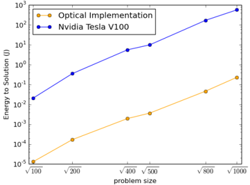
The image is a line graph comparing the energy consumption (in Joules) required to solve a problem of varying sizes for two different computational implementations: an "Optical Implementation" and an "Nvidia Tesla V100" (a GPU). The graph uses a logarithmic scale for the vertical axis (energy) and a linear scale for the horizontal axis (problem size, expressed as square roots).
### Components/Axes
* **Chart Type:** Line graph with markers.
* **X-Axis (Horizontal):**
* **Label:** `problem size`
* **Scale/Ticks:** Linear scale with categorical markers at `√100`, `√200`, `√400`, `√500`, `√800`, `√1000`.
* **Y-Axis (Vertical):**
* **Label:** `Energy to Solution (J)`
* **Scale/Ticks:** Logarithmic scale (base 10). Major ticks are labeled at `10^-5`, `10^-4`, `10^-3`, `10^-2`, `10^-1`, `10^0`, `10^1`, `10^2`, `10^3`.
* **Legend:**
* **Position:** Top-left corner of the plot area.
* **Entry 1:** `Optical Implementation` - Represented by an orange line with circular markers.
* **Entry 2:** `Nvidia Tesla V100` - Represented by a blue line with circular markers.
### Detailed Analysis
**Data Series 1: Optical Implementation (Orange Line)**
* **Trend:** The line slopes consistently upward from left to right, indicating energy consumption increases with problem size.
* **Data Points (Approximate):**
* At `√100`: ~10^-5 J
* At `√200`: ~10^-4 J
* At `√400`: ~10^-3 J
* At `√500`: Slightly above 10^-3 J (approx. 2-3 x 10^-3 J)
* At `√800`: ~10^-2 J
* At `√1000`: ~10^-1 J
**Data Series 2: Nvidia Tesla V100 (Blue Line)**
* **Trend:** The line also slopes consistently upward from left to right, showing a similar increasing trend but at a much higher energy level.
* **Data Points (Approximate):**
* At `√100`: ~10^-2 J
* At `√200`: ~10^0 J (1 Joule)
* At `√400`: ~10^1 J (10 Joules)
* At `√500`: Slightly above 10^1 J (approx. 2-3 x 10^1 J)
* At `√800`: ~10^2 J (100 Joules)
* At `√1000`: ~10^3 J (1000 Joules)
### Key Observations
1. **Consistent Energy Gap:** The blue line (Nvidia V100) is consistently positioned 2-3 orders of magnitude (100x to 1000x) higher on the logarithmic y-axis than the orange line (Optical Implementation) for every corresponding problem size.
2. **Parallel Trends:** Both lines appear roughly parallel on this log-linear plot, suggesting that the *rate* of increase in energy consumption relative to problem size is similar for both implementations, even though their absolute energy values are vastly different.
3. **No Crossover:** The lines do not intersect within the plotted range. The Optical Implementation maintains its energy advantage across all tested problem sizes.
4. **Data Density:** Data points are provided at six discrete problem sizes, with a slightly closer spacing between `√400` and `√500`.
### Interpretation
This graph presents a compelling case for the energy efficiency of the "Optical Implementation" compared to a high-performance electronic GPU (Nvidia Tesla V100) for the given computational task.
* **Core Message:** The optical approach is dramatically more energy-efficient, requiring roughly 100 to 1000 times less energy to solve problems of the same size. This is the primary takeaway.
* **Scalability:** The parallel upward trends indicate that while both systems consume more energy for larger problems, the optical system's energy cost scales in a similar *proportional* manner but from a vastly lower baseline. This suggests the fundamental advantage is architectural, not just a fixed offset.
* **Contextual Implication:** For applications where energy consumption is a critical constraint (e.g., large-scale data centers, edge computing, or sustainability-focused projects), the optical implementation presents a potentially transformative alternative. The graph quantifies the magnitude of that potential advantage.
* **Limitations of the View:** The graph does not specify the nature of the "problem," the time taken for the solution, or other performance metrics like accuracy. It isolates and compares only the energy dimension. The use of `√` on the x-axis suggests the underlying problem dimension might be the square of the plotted values (e.g., a 100x100 matrix at `√100`).