## Diagram: Set Representation ### Overview The image is a diagram representing two sets, Q and L, within a larger space defined by axes n0 and n1. The sets are visually distinguished by color (red for Q, yellow for L) and are positioned within a grid-like structure. The diagram illustrates the relationship and overlap between these sets. ### Components/Axes * **Axes:** * Horizontal axis: n0 * Vertical axis: n1 * **Sets:** * Q: Represented by a red area. * L: Represented by a yellow area. * **Grid:** Dashed lines forming a grid structure. * **Background:** Gray area representing the overall space. ### Detailed Analysis * **Set Q:** The red area representing set Q occupies a significant portion of the space, primarily on the left side. It extends vertically from approximately 0.1 to 1 on the n1 axis and horizontally from approximately 0.1 to 0.6 on the n0 axis. * **Set L:** The yellow area representing set L is positioned on the right side of the diagram. It extends vertically from approximately 0.3 to 0.9 on the n1 axis and horizontally from approximately 0.6 to 1 on the n0 axis. * **Overlap:** There is a small region where the red and yellow areas overlap, indicating the intersection of sets Q and L. This overlap occurs approximately between 0.6 and 0.7 on the n0 axis and 0.3 and 0.9 on the n1 axis. * **Grid:** The dashed grid lines provide a visual reference for the position and extent of the sets. The grid lines are spaced approximately equally along both axes. ### Key Observations * Sets Q and L have a partial overlap, indicating some common elements. * Set Q is positioned more towards the left side of the space, while set L is positioned more towards the right. * The gray background defines the boundaries of the overall space. ### Interpretation The diagram visually represents the relationship between two sets, Q and L, within a defined space. The overlap between the sets indicates a non-empty intersection, meaning there are elements that belong to both sets. The positioning of the sets relative to the axes and each other provides a spatial understanding of their distribution and relationship within the overall space. The grid helps to visualize the relative sizes and positions of the sets. The diagram is a visual aid to understand set theory concepts.

\n ## Diagram: Phase Diagram Representation ### Overview The image depicts a two-dimensional diagram representing a phase space or a region divided into different phases. The diagram uses color-coding to distinguish between different regions, labeled 'Q' and 'L'. The axes are labeled 'n₀' and 'n₁'. The diagram appears to illustrate a conceptual partitioning of a space based on two variables. ### Components/Axes * **Axes:** * Horizontal axis: labeled 'n₀' * Vertical axis: labeled 'n₁' * **Regions:** * Yellow region: Labeled 'L' in the center-right. * Pink/Red region: Labeled 'Q' in the center-left. * Gray region: Surrounding the pink and yellow regions, forming a border along the axes. * **Grid:** Dashed lines create a grid pattern within the diagram, dividing the regions into smaller squares. ### Detailed Analysis or Content Details The diagram shows a rectangular area defined by the axes n₀ and n₁. The area is partitioned into three distinct regions: * **Region Q (Pink/Red):** Occupies the left half of the rectangle. It is further divided into 9 equal squares by the dashed grid lines. * **Region L (Yellow):** Occupies the right half of the rectangle. It is also divided into 9 equal squares by the dashed grid lines. * **Gray Region:** Forms a border around the pink and yellow regions, extending along the n₀ and n₁ axes. This region appears to represent a boundary or transition zone. There are no numerical values provided on the axes, so the scale and range of n₀ and n₁ are unknown. The diagram is purely qualitative, illustrating the relative positions and areas of the different regions. ### Key Observations * The diagram visually represents two distinct phases, 'Q' and 'L', separated by a boundary. * The areas of regions 'Q' and 'L' appear to be equal, each occupying approximately half of the total area. * The gray region suggests a transition or boundary between the two phases. * The grid lines indicate a uniform partitioning of the space within each phase. ### Interpretation This diagram likely represents a phase diagram in a physical or chemical system. The variables n₀ and n₁ could represent concentrations, temperature, pressure, or other relevant parameters. The regions 'Q' and 'L' represent different phases of the system, and the gray region represents a phase boundary where the two phases coexist. The equal areas of 'Q' and 'L' might suggest that the two phases are equally probable or stable under the conditions represented by the diagram. The grid lines could indicate a discrete or quantized nature of the system. Without further context, it is difficult to determine the specific meaning of the diagram. However, it clearly illustrates a partitioning of a space into different phases based on two variables. The diagram is a conceptual representation and does not provide any quantitative data. It is a schematic illustration of a system's state space.

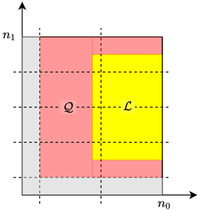
\n ## Diagram: Parameter Space Partitioning ### Overview The image displays a two-dimensional Cartesian coordinate system diagram that partitions a parameter space defined by axes \( n_0 \) and \( n_1 \) into distinct, colored rectangular regions. The diagram visually represents the relationship or containment between different sets or categories labeled \( Q \) and \( \mathcal{L} \). ### Components/Axes * **Axes:** * **Horizontal Axis (X-axis):** Labeled \( n_0 \). An arrow points to the right, indicating the positive direction. * **Vertical Axis (Y-axis):** Labeled \( n_1 \). An arrow points upward, indicating the positive direction. * **Grid:** The plot area is subdivided by a grid of dashed black lines, creating a 4x4 matrix of smaller rectangular cells. These lines serve as reference boundaries but are not labeled with specific numerical values. * **Regions & Labels:** The space is divided into three primary colored regions: 1. **Gray Region:** A vertical rectangular strip occupying the leftmost portion of the plot, spanning the full height of the \( n_1 \) axis. It is unlabeled. 2. **Pink Region:** A larger rectangular area to the right of the gray region. It spans most of the remaining width and the full height. It is labeled with the letter **\( Q \)**, placed in its center-left area. 3. **Yellow Region:** A smaller rectangular area nested within the pink region, positioned towards the right side. It is labeled with the script letter **\( \mathcal{L} \)**, placed in its center. ### Detailed Analysis * **Spatial Relationships & Boundaries:** * The **gray region** is defined by \( n_0 \) values from the origin (0) to the first vertical dashed grid line. * The **pink region (\( Q \))** begins at the first vertical grid line and extends to the right edge of the plot. It covers all values of \( n_1 \). * The **yellow region (\( \mathcal{L} \))** is a strict subset of the pink region. Its left boundary aligns with the third vertical grid line, and its right boundary aligns with the plot's right edge. Its bottom boundary aligns with the second horizontal grid line from the bottom, and its top boundary aligns with the top edge of the plot (the \( n_1 \) axis maximum). * **Containment Hierarchy:** The diagram clearly shows a containment relationship: \( \mathcal{L} \subset Q \). The set \( \mathcal{L} \) is entirely contained within the set \( Q \), which in turn is contained within the full plotted space (excluding the gray region). ### Key Observations 1. **Asymmetric Partitioning:** The space is not divided equally. The gray region is a narrow strip, the pink region is large, and the yellow region is a significant but smaller subset of the pink. 2. **Axis-Aligned Boundaries:** All region boundaries are perfectly vertical or horizontal, aligned with the axes and the implicit grid. This suggests the partitioning is based on independent thresholds or ranges for the parameters \( n_0 \) and \( n_1 \). 3. **Unlabeled Gray Zone:** The gray region lacks a label, implying it may represent a default, excluded, or baseline condition separate from the categorized sets \( Q \) and \( \mathcal{L} \). ### Interpretation This diagram is a conceptual visualization of set relationships within a two-parameter space (\( n_0, n_1 \)). It is likely used in fields like machine learning, optimization, or control theory to illustrate: * **Feasible Regions:** \( Q \) could represent a broad feasible set of parameters, while \( \mathcal{L} \) represents a more constrained, optimal, or target subset within it. * **Classification Boundaries:** The regions could demarcate different classes or modes of system behavior based on the values of \( n_0 \) and \( n_1 \). The gray area might be an "invalid" or "other" class. * **Algorithm Phases:** It could depict the progression of an algorithm, where the search space narrows from the full plot, to \( Q \), and finally to the solution region \( \mathcal{L} \). The absence of numerical values on the grid lines indicates this is a schematic, meant to convey topological relationships (containment, adjacency) rather than precise quantitative data. The core message is the hierarchical inclusion of \( \mathcal{L} \) within \( Q \) across the defined parameter space.

## Heatmap/Diagram: Partitioned Grid with Colored Regions ### Overview The image depicts a partitioned grid with two distinct colored regions labeled **Q** (red) and **L** (yellow), separated by dashed vertical and horizontal lines. The grid is bounded by axes labeled **n₀** (horizontal) and **n₁** (vertical), with no explicit numerical scale provided. A legend in the top-right corner associates colors with labels. ### Components/Axes - **Axes**: - **n₀**: Horizontal axis, labeled at the bottom-right corner. - **n₁**: Vertical axis, labeled at the top-left corner. - **Legend**: - **Red**: Labeled **Q** (top-left region). - **Yellow**: Labeled **L** (bottom-right region). - **Grid Structure**: - Dashed vertical lines divide the grid into three vertical sections. - Dashed horizontal lines divide the grid into five horizontal sections. ### Detailed Analysis 1. **Region Q (Red)**: - Occupies the leftmost vertical section (n₀ ≈ 0 to 0.6). - Spans horizontally from n₁ ≈ 0.2 to 0.8. - Includes a small yellow "L" region embedded within its lower-right quadrant. 2. **Region L (Yellow)**: - Occupies the rightmost vertical section (n₀ ≈ 0.6 to 1). - Spans horizontally from n₁ ≈ 0.2 to 0.8. - Overlaps with the red "Q" region in its upper-left quadrant. 3. **Gray Borders**: - Thin gray regions occupy the outermost edges of the grid (n₀ ≈ 0–0.1 and n₀ ≈ 0.9–1; n₁ ≈ 0–0.1 and n₁ ≈ 0.9–1). ### Key Observations - **Overlap**: The yellow "L" region partially overlaps with the red "Q" region in the lower-right quadrant of Q. - **Spatial Distribution**: - Q dominates the left side of the grid. - L dominates the right side but is constrained vertically between n₁ ≈ 0.2 and 0.8. - **Legend Consistency**: Colors in the legend (red for Q, yellow for L) match the regions in the grid. ### Interpretation This diagram likely represents a spatial partitioning of a system or dataset into two primary categories (**Q** and **L**), with overlapping regions suggesting potential interactions or dependencies. The absence of numerical values on the axes implies the focus is on categorical or qualitative relationships rather than quantitative measurements. The embedded "L" within "Q" could indicate a hierarchical or nested relationship between the two categories. The gray borders may represent boundaries or thresholds outside the primary operational range of Q and L.