## Chart: Convergence of Estimators
### Overview
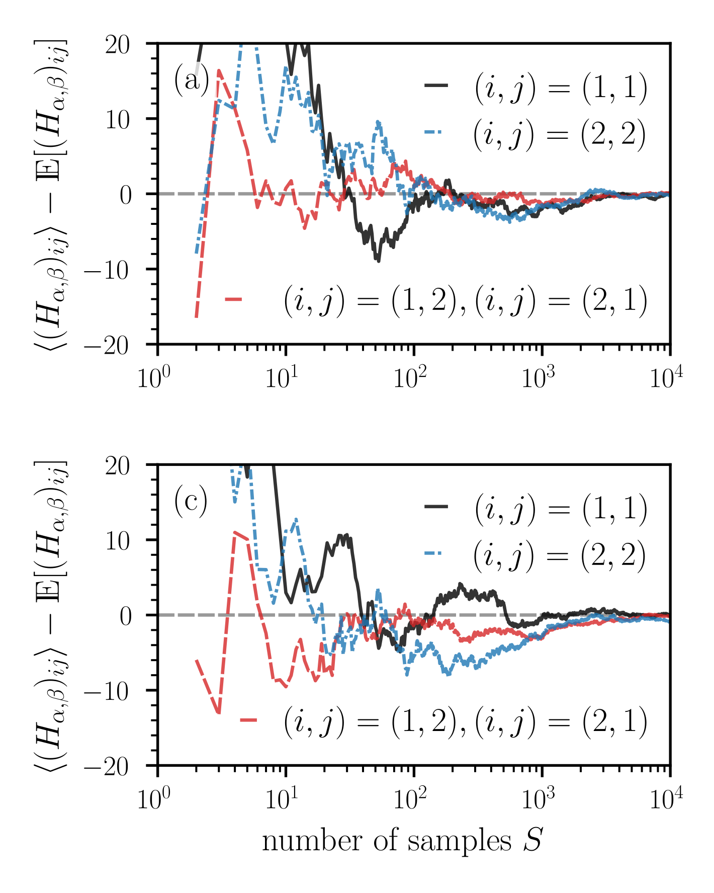
The image contains two line charts, labeled (a) and (c), displaying the convergence behavior of estimators as the number of samples increases. The y-axis represents the difference between the estimator and its expected value, while the x-axis represents the number of samples on a logarithmic scale. Three different data series are plotted in each chart, corresponding to different index pairs (i, j).
### Components/Axes
* **Chart Titles:** (a) and (c) in the top-left corner of each chart.
* **Y-axis Label:** "⟨⟨(Hα,β)ij⟩⟩ – E[(Hα,β)ij]" for both charts. The y-axis ranges from -20 to 20 with tick marks at -20, -10, 0, 10, and 20.
* **X-axis Label:** "number of samples S" for the bottom chart. The x-axis is a logarithmic scale ranging from 10^0 to 10^4, with tick marks at 10^0, 10^1, 10^2, 10^3, and 10^4.
* **Horizontal Dashed Line:** A gray dashed line is present at y = 0 on both charts.
* **Legend:** Located in the top-right of each chart.
* Black solid line: (i, j) = (1, 1)
* Blue dashed line: (i, j) = (2, 2)
* Red dashed line: (i, j) = (1, 2), (i, j) = (2, 1)
### Detailed Analysis
**Chart (a):**
* **(i, j) = (1, 1) (Black solid line):** Starts around y=20 at x=10^0, fluctuates significantly between 10^0 and 10^2, and then converges towards 0 as the number of samples increases to 10^4.
* **(i, j) = (2, 2) (Blue dashed line):** Starts around y= -10 at x=10^0, fluctuates significantly between 10^0 and 10^2, and then converges towards 0 as the number of samples increases to 10^4.
* **(i, j) = (1, 2), (i, j) = (2, 1) (Red dashed line):** Starts around y=-15 at x=10^0, fluctuates significantly between 10^0 and 10^2, and then converges towards 0 as the number of samples increases to 10^4.
**Chart (c):**
* **(i, j) = (1, 1) (Black solid line):** Starts around y=0 at x=10^0, fluctuates significantly between 10^0 and 10^2, and then converges towards 0 as the number of samples increases to 10^4.
* **(i, j) = (2, 2) (Blue dashed line):** Starts around y= -10 at x=10^0, fluctuates significantly between 10^0 and 10^2, and then converges towards 0 as the number of samples increases to 10^4.
* **(i, j) = (1, 2), (i, j) = (2, 1) (Red dashed line):** Starts around y=-15 at x=10^0, fluctuates significantly between 10^0 and 10^2, and then converges towards 0 as the number of samples increases to 10^4.
### Key Observations
* All three data series in both charts converge towards 0 as the number of samples increases.
* The fluctuations are more pronounced at lower sample sizes (between 10^0 and 10^2).
* The convergence rate appears to be similar for all three data series in each chart.
* Chart (a) and (c) show similar convergence behavior for the same (i,j) values.
### Interpretation
The charts demonstrate the convergence of estimators to their expected values as the number of samples increases. The fluctuations at lower sample sizes indicate higher variance in the estimates, which decreases as more data is used. The convergence towards 0 suggests that the estimators are unbiased. The similarity between charts (a) and (c) suggests that the underlying process being estimated is consistent across different conditions or parameters represented by (a) and (c). The data suggests that a larger number of samples is required to obtain more accurate and reliable estimates.