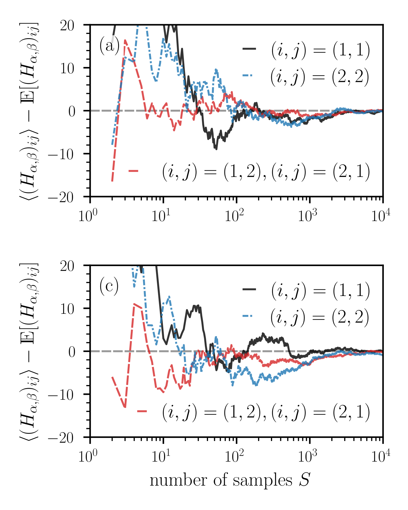
## Line Graphs: Expectation Difference vs. Number of Samples ### Overview The image contains two identical line graphs (labeled (a) and (c)) comparing the difference between ⟨(H_α,β)_ij⟩ and E[(H_α,β)_ij] across three (i,j) pairs: (1,1), (2,2), and (1,2)/(2,1). Both graphs share the same axes, labels, and data trends, with minor visual differences in line placement. --- ### Components/Axes - **X-axis**: "number of samples S" (logarithmic scale: 10⁰ to 10⁴) - **Y-axis**: ⟨(H_α,β)_ij⟩ − E[(H_α,β)_ij] (range: -20 to 20) - **Legends**: - Solid black line: (i,j) = (1,1) - Dashed blue line: (i,j) = (2,2) - Dashed red line: (i,j) = (1,2), (i,j) = (2,1) - **Placement**: Legends are positioned in the top-right corner of each graph. --- ### Detailed Analysis #### Graph (a) - **Solid black line (1,1)**: - Starts at ~15 at S=10⁰, dips below zero (~−10) at S=10¹, then stabilizes near zero by S=10³. - Peak-to-trough oscillation amplitude decreases with increasing S. - **Dashed blue line (2,2)**: - Begins at ~5 at S=10⁰, fluctuates between −5 and 15, converging to zero by S=10³. - Shows sharper oscillations than the (1,1) line. - **Dashed red line (1,2)/(2,1)**: - Starts at ~−15 at S=10⁰, rises to ~5 by S=10², then stabilizes near zero. - Largest initial deviation among all lines. #### Graph (c) - **Solid black line (1,1)**: - Similar to (a), but converges to zero slightly earlier (by S=10².5). - **Dashed blue line (2,2)**: - Mirrors (a) but with reduced oscillation amplitude. - **Dashed red line (1,2)/(2,1)**: - Converges to zero faster than in (a), reaching stability by S=10². --- ### Key Observations 1. **Convergence**: All lines converge to zero as S increases, with faster convergence in graph (c). 2. **Initial Deviations**: - (1,1) pair starts highest but stabilizes fastest. - (1,2)/(2,1) pair exhibits the largest initial negative deviation. 3. **Oscillation Patterns**: - (2,2) pair shows the most pronounced oscillations before stabilization. 4. **Graph (a) vs. (c)**: - Graph (c) demonstrates earlier convergence across all (i,j) pairs. --- ### Interpretation The data suggests that increasing the number of samples (S) reduces the discrepancy between the expected value E[(H_α,β)_ij] and the observed expectation ⟨(H_α,β)_ij⟩. This implies: - **Stability**: Larger sample sizes lead to more consistent measurements, aligning with statistical principles of reduced variance. - **Parameter Sensitivity**: - The (1,1) pair’s rapid stabilization may indicate lower sensitivity to sampling noise. - The (1,2)/(2,1) pair’s delayed convergence suggests higher sensitivity to initial conditions or parameter interactions. - **Graph (c) Insights**: Faster convergence in (c) could reflect optimized system parameters or reduced noise in the modeled scenario. The trends highlight the importance of sample size in achieving reliable estimates, particularly for systems with complex parameter dependencies (e.g., (1,2)/(2,1) pairs).