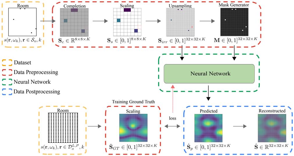
## Flowchart: Neural Network Training Pipeline for Spatial Data Processing ### Overview The diagram illustrates a machine learning pipeline for processing spatial data (likely room layouts or occupancy patterns) through a neural network. It shows data flow from raw input to model output, including preprocessing, training, and postprocessing stages. Key components include data transformation steps, neural network architecture, and evaluation metrics. ### Components/Axes **Legend (Left Side):** - **Dataset**: Orange dashed box (raw input data) - **Data Preprocessing**: Red dashed box (transformations) - **Neural Network**: Green dashed box (core model) - **Data Postprocessing**: Blue dashed box (output refinement) **Main Components:** 1. **Input Stage (Top Left):** - **Room**: Represented as a grid with coordinates `(r, ω_k)` and parameters `s(r, ω_k), r ∈ S_o, k` - **Completion**: 8×8×K grid (`S_c ∈ ℝ^8×8×K`) with missing data (gray squares) - **Scaling**: Normalized to `[0,1]^8×8×K` (`S_s`) - **Upsampling**: Expanded to 32×32×K grid (`S_irr`) - **Mask Generator**: Binary mask `M ∈ {0,1}^32×32×K` (black/white squares) 2. **Neural Network (Center):** - Takes `S_irr` and `M` as inputs - Outputs predicted values `Ŝ_p ∈ [0,1]^32×32×K` 3. **Output Stage (Bottom Right):** - **Training Ground Truth**: Heatmap `S_GT ∈ [0,1]^32×32×K` (reference data) - **Predicted**: Heatmap `Ŝ_p` (model output) - **Reconstructed**: Final output `Ŝ ∈ ℝ^32×32×K` **Arrows & Flow:** - Red arrows: Data preprocessing steps - Green arrows: Neural network processing - Blue arrows: Postprocessing steps - Loss function connects predicted vs. ground truth ### Detailed Analysis **Dataset Section:** - Raw room data represented as sparse grid with coordinates `(r, ω_k)` - Parameters include `s(r, ω_k)` (possibly occupancy values) and `r ∈ S_o, k` (room-specific constraints) **Preprocessing Pipeline:** 1. **Completion**: Fills missing data in 8×8×K grid (visualized as gray squares) 2. **Scaling**: Normalizes values to [0,1] range 3. **Upsampling**: Increases resolution from 8×8 to 32×32 while maintaining K channels 4. **Masking**: Creates binary mask to highlight relevant regions **Neural Network:** - Input dimensions: 32×32×K (spatial + channel dimensions) - Output dimensions match training ground truth (32×32×K) - Loss function measures discrepancy between predicted (`Ŝ_p`) and ground truth (`S_GT`) **Postprocessing:** - Reconstructed output `Ŝ` in real-valued space (ℝ^32×32×K) - Heatmaps show spatial distribution of values (likely occupancy probabilities) ### Key Observations 1. **Dimensionality Progression**: - Input: 8×8×K → Preprocessed: 32×32×K - Suggests multi-scale processing with spatial enhancement 2. **Masking Mechanism:** - Binary mask `M` likely focuses network attention on critical regions - Visualized as black/white squares in 32×32 grid 3. **Heatmap Interpretation:** - Training Ground Truth (`S_GT`): Ground truth occupancy patterns - Predicted (`Ŝ_p`): Model's probability estimates - Reconstructed (`Ŝ`): Final output after postprocessing 4. **Loss Function:** - Direct comparison between predicted and ground truth heatmaps - Implies pixel-wise error minimization (e.g., MSE or cross-entropy) ### Interpretation This pipeline demonstrates a spatial data processing workflow for occupancy prediction or room layout reconstruction. The preprocessing steps address data sparsity (completion) and scale mismatch (upsampling), while the mask generator enables focused learning on relevant regions. The neural network's ability to match ground truth heatmaps suggests it's trained for tasks like occupancy estimation or spatial reconstruction. The use of 32×32×K dimensions indicates the model handles multi-channel spatial data (e.g., RGB + depth), with K representing additional modalities. The loss function's direct comparison implies the model is optimized for high-resolution spatial accuracy, potentially for applications in smart buildings, robotics navigation, or architectural design. Notable design choices include: - Progressive resolution increase (8→32) for feature learning - Binary masking for attention mechanism - Heatmap visualization for model output interpretation - Real-valued reconstruction suggesting continuous output space