## Chart: Gradient Updates vs. Dimension
### Overview
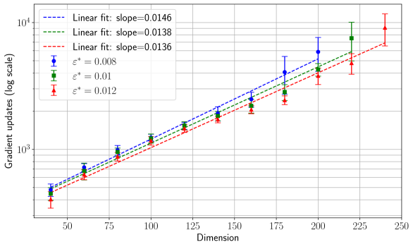
The image presents a chart illustrating the relationship between the dimension of a space and the number of gradient updates required, displayed on a logarithmic scale. Three different curves are plotted, each representing a different value of epsilon (ε), a parameter likely related to the optimization process. Error bars are included for each data point, indicating the variability or uncertainty in the gradient update measurements. Linear fits are shown for each curve, with their corresponding slopes provided.
### Components/Axes
* **X-axis:** Dimension, ranging from approximately 50 to 250.
* **Y-axis:** Gradient updates (log scale), ranging from approximately 10^3 to 10^4.
* **Legend:** Located in the top-left corner, containing the following entries:
* Blue Line with Circle Markers: ε* = 0.008, Linear fit: slope=0.0146
* Green Line with Square Markers: ε* = 0.01, Linear fit: slope=0.0138
* Red Line with Triangle Markers: ε* = 0.012, Linear fit: slope=0.0136
* **Linear Fits:** Dashed lines corresponding to each data series, with the slope of the fit indicated in the legend.
* **Error Bars:** Vertical lines extending above and below each data point, representing the uncertainty in the gradient update measurements.
### Detailed Analysis
The chart displays three data series, each representing a different epsilon value. All three series show a generally upward trend, indicating that the number of gradient updates increases with increasing dimension. The error bars suggest some variability in the measurements, but the overall trend is clear.
Let's extract approximate data points, noting the logarithmic scale of the Y-axis:
**1. ε* = 0.008 (Blue Line):**
* Dimension = 50: Gradient Updates ≈ 10^3.1 (≈ 1259)
* Dimension = 75: Gradient Updates ≈ 10^3.3 (≈ 1995)
* Dimension = 100: Gradient Updates ≈ 10^3.5 (≈ 3162)
* Dimension = 125: Gradient Updates ≈ 10^3.65 (≈ 4467)
* Dimension = 150: Gradient Updates ≈ 10^3.8 (≈ 6310)
* Dimension = 175: Gradient Updates ≈ 10^3.9 (≈ 7943)
* Dimension = 200: Gradient Updates ≈ 10^4.0 (≈ 10000)
* Dimension = 225: Gradient Updates ≈ 10^4.1 (≈ 12589)
**2. ε* = 0.01 (Green Line):**
* Dimension = 50: Gradient Updates ≈ 10^3.2 (≈ 1585)
* Dimension = 75: Gradient Updates ≈ 10^3.4 (≈ 2512)
* Dimension = 100: Gradient Updates ≈ 10^3.6 (≈ 3981)
* Dimension = 125: Gradient Updates ≈ 10^3.7 (≈ 5012)
* Dimension = 150: Gradient Updates ≈ 10^3.85 (≈ 7079)
* Dimension = 175: Gradient Updates ≈ 10^4.0 (≈ 10000)
* Dimension = 200: Gradient Updates ≈ 10^4.1 (≈ 12589)
* Dimension = 225: Gradient Updates ≈ 10^4.2 (≈ 15849)
**3. ε* = 0.012 (Red Line):**
* Dimension = 50: Gradient Updates ≈ 10^3.0 (≈ 1000)
* Dimension = 75: Gradient Updates ≈ 10^3.2 (≈ 1585)
* Dimension = 100: Gradient Updates ≈ 10^3.4 (≈ 2512)
* Dimension = 125: Gradient Updates ≈ 10^3.55 (≈ 3548)
* Dimension = 150: Gradient Updates ≈ 10^3.7 (≈ 5012)
* Dimension = 175: Gradient Updates ≈ 10^3.85 (≈ 7079)
* Dimension = 200: Gradient Updates ≈ 10^4.0 (≈ 10000)
* Dimension = 225: Gradient Updates ≈ 10^4.15 (≈ 14125)
### Key Observations
* The number of gradient updates increases linearly with dimension for all three epsilon values.
* Higher epsilon values (ε* = 0.012) generally require fewer gradient updates for a given dimension compared to lower epsilon values (ε* = 0.008).
* The slopes of the linear fits are relatively similar, ranging from 0.0136 to 0.0146.
* The error bars indicate that the measurements are not perfectly precise, but the trends are still clear.
### Interpretation
The chart suggests that the number of gradient updates needed to converge during optimization scales linearly with the dimension of the problem space. This is a significant observation, as it implies that optimization becomes increasingly expensive as the dimensionality increases. The different curves for different epsilon values suggest that the choice of epsilon can influence the number of updates required. Larger epsilon values may allow for faster initial progress but could potentially lead to instability or suboptimal solutions. The relatively small differences in the slopes of the linear fits indicate that the scaling behavior is fairly consistent across the tested epsilon values. The logarithmic scale on the Y-axis emphasizes the exponential growth in gradient updates as the dimension increases, highlighting the challenges of optimizing high-dimensional spaces. This data could be used to inform the selection of appropriate optimization algorithms and parameters for different dimensionality problems. The error bars suggest that the relationship is not perfectly deterministic, and further investigation may be needed to understand the sources of variability.