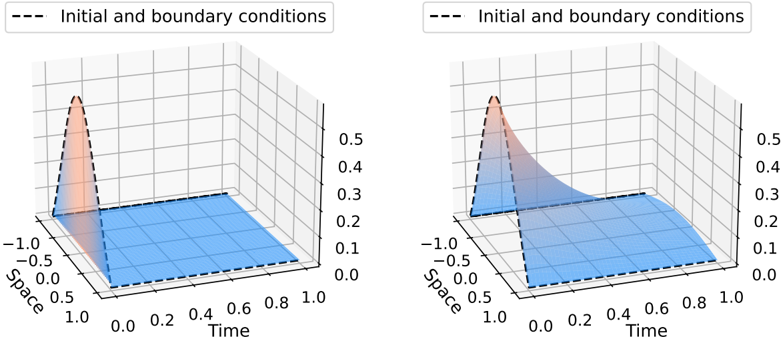
## 3D Surface Plots: Time Evolution of a Distribution ### Overview The image consists of two 3D surface plots, side-by-side, visualizing the evolution of a distribution over time and space. Both plots share the same axes: "Time" (x-axis), "Space" (y-axis), and an unnamed z-axis representing the magnitude of the distribution. The left plot shows the initial state, while the right plot shows a later state. The initial and boundary conditions are outlined with a dashed black line. ### Components/Axes * **X-axis:** "Time", ranging from 0.0 to 1.0 in increments of 0.2. * **Y-axis:** "Space", ranging from -1.0 to 1.0 in increments of 0.5. * **Z-axis:** No explicit label, but represents the magnitude/value of the distribution, ranging from 0.0 to 0.5 in increments of 0.1. * **Legend:** "Initial and boundary conditions" represented by a dashed black line. Located at the top of each plot. * **Surface:** The surface is colored blue, with a peak colored orange/red. ### Detailed Analysis **Left Plot (Initial State):** * The distribution is highly localized at a specific point in space (around -0.8 to -1.0) at time 0. * The peak value of the distribution is approximately 0.5. * The distribution is essentially zero for all other spatial locations and times. * The initial and boundary conditions are marked by a dashed black line, outlining the base and the peak of the distribution. **Right Plot (Later State):** * The distribution has spread out over time. * The peak value has decreased to approximately 0.3-0.4. * The distribution is no longer localized but is spread across a range of spatial locations. * The initial and boundary conditions are marked by a dashed black line, outlining the base of the distribution. ### Key Observations * The distribution diffuses or spreads out over time. * The peak value of the distribution decreases as it spreads. * The initial condition is a sharp peak, which smooths out over time. ### Interpretation The plots likely represent the solution to a diffusion equation or a similar partial differential equation. The left plot shows the initial condition, where a quantity is concentrated at a single point in space. The right plot shows how that quantity spreads out over time due to diffusion. The decrease in the peak value is consistent with the conservation of the total quantity, as the initial amount spreads over a larger area. The dashed black line represents the constraints or limits of the system.