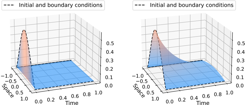
## 3D Surface Plots: Initial vs Evolved Boundary Conditions ### Overview Two side-by-side 3D surface plots compare spatial-temporal dynamics under different boundary conditions. Both plots share identical axis labels but differ in surface morphology and color coding. The left plot shows a localized peak, while the right demonstrates a diffusing wavefront. ### Components/Axes - **X-axis (Space)**: -1.0 to 1.0 in 0.1 increments - **Y-axis (Time)**: 0.0 to 1.0 in 0.1 increments - **Z-axis (Amplitude)**: 0.0 to 0.5 in 0.1 increments - **Legend**: Dashed lines represent "Initial and boundary conditions" - **Color coding**: - Left plot: Red dashed lines (initial conditions) - Right plot: Blue gradient surface (evolved conditions) ### Detailed Analysis **Left Plot**: - Red dashed line forms a triangular peak at: - Space = 0.0 - Time = 0.2 - Amplitude = 0.5 - Base plane remains at Z=0.0 except at peak location - No intermediate values between peak and base **Right Plot**: - Blue gradient surface originates from same peak location: - Space = 0.0 - Time = 0.2 - Amplitude = 0.5 - Surface spreads radially outward: - At Time = 0.4: Amplitude ≈ 0.3 at Space = ±0.2 - At Time = 0.6: Amplitude ≈ 0.2 at Space = ±0.4 - Base plane remains Z=0.0 except under propagating wavefront ### Key Observations 1. **Peak Consistency**: Both plots share identical initial peak coordinates (Space=0.0, Time=0.2, Amplitude=0.5) 2. **Temporal Evolution**: Right plot shows amplitude decay (0.5→0.2 over Time=0.2→0.6) with spatial dispersion 3. **Boundary Condition Impact**: Left plot maintains sharp peak; right plot demonstrates wavefront propagation/diffusion 4. **Color Correlation**: Red (left) vs Blue (right) confirms distinct condition sets per legend ### Interpretation The plots visualize wave propagation under contrasting boundary conditions: - **Left Plot**: Represents a fixed-end boundary condition where the initial disturbance (peak) remains localized but stationary - **Right Plot**: Illustrates free-end or dissipative boundary conditions causing the wavefront to: - Propagate outward at ~0.2 space units per time unit - Experience amplitude attenuation (50% reduction over 0.4 time units) - Maintain energy conservation through spatial dispersion The identical initial conditions with divergent temporal evolution highlight how boundary constraints fundamentally alter system behavior. The right plot's gradient surface suggests a continuous wave equation solution, while the left plot's dashed lines imply discrete boundary reflections.