## Scatter Plot Comparison: Unstructured vs. Structured Data
### Overview
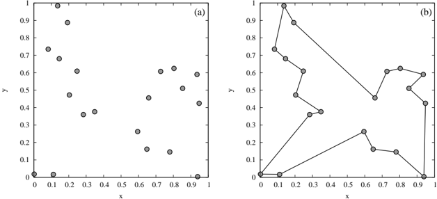
The image displays two side-by-side scatter plots, labeled (a) and (b), sharing identical axes. Plot (a) shows a set of discrete, unconnected data points. Plot (b) shows the same set of points, but with a subset of them connected by straight lines, forming a continuous, non-intersecting path or tour. The image appears to be a figure from a technical or scientific document, likely illustrating a concept in data analysis, optimization (e.g., Traveling Salesman Problem), or graph theory.
### Components/Axes
* **Chart Type:** Two-panel scatter plot with an overlay of connecting lines in panel (b).
* **Panel Labels:** "(a)" in the top-right corner of the left plot; "(b)" in the top-right corner of the right plot.
* **Axes (Both Panels):**
* **X-axis:** Labeled "x". Scale ranges from 0 to 1. Major tick marks and labels at 0, 0.1, 0.2, 0.3, 0.4, 0.5, 0.6, 0.7, 0.8, 0.9, 1.
* **Y-axis:** Labeled "y". Scale ranges from 0 to 1. Major tick marks and labels at 0, 0.1, 0.2, 0.3, 0.4, 0.5, 0.6, 0.7, 0.8, 0.9, 1.
* **Data Points:** Represented by gray-filled circles with black outlines. The same set of points appears in both panels.
* **Legend:** None present.
* **Spatial Layout:** The two plots are arranged horizontally. Plot (a) occupies the left half, Plot (b) the right half. The axes frames are identical in size and position within their respective halves.
### Detailed Analysis
**Panel (a): Unconnected Scatter Points**
* **Trend:** No inherent order or connection is shown. The points appear to be distributed in a somewhat clustered but irregular pattern across the unit square.
* **Data Point Extraction (Approximate Coordinates):**
* (0.00, 0.00)
* (0.10, 0.00)
* (0.10, 0.73)
* (0.15, 1.00)
* (0.18, 0.68)
* (0.20, 0.47)
* (0.25, 0.61)
* (0.30, 0.36)
* (0.35, 0.38)
* (0.60, 0.26)
* (0.62, 0.45)
* (0.65, 0.16)
* (0.75, 0.14)
* (0.75, 0.61)
* (0.80, 0.62)
* (0.85, 0.51)
* (0.90, 0.59)
* (0.95, 0.42)
* (0.95, 0.00)
**Panel (b): Connected Path**
* **Trend:** A single, continuous path is drawn connecting 18 of the 19 points from panel (a). The path does not intersect itself. It starts at (0.00, 0.00), traverses the points in a specific order, and ends at (0.95, 0.00). The point at (0.10, 0.00) is **not** included in the path.
* **Path Sequence (Approximate Order):** The visual path suggests the following connection order:
1. (0.00, 0.00) → (0.10, 0.73)
2. (0.10, 0.73) → (0.15, 1.00)
3. (0.15, 1.00) → (0.18, 0.68)
4. (0.18, 0.68) → (0.25, 0.61)
5. (0.25, 0.61) → (0.20, 0.47)
6. (0.20, 0.47) → (0.30, 0.36)
7. (0.30, 0.36) → (0.35, 0.38)
8. (0.35, 0.38) → (0.62, 0.45)
9. (0.62, 0.45) → (0.60, 0.26)
10. (0.60, 0.26) → (0.65, 0.16)
11. (0.65, 0.16) → (0.75, 0.14)
12. (0.75, 0.14) → (0.95, 0.00)
13. (0.95, 0.00) → (0.95, 0.42)
14. (0.95, 0.42) → (0.90, 0.59)
15. (0.90, 0.59) → (0.85, 0.51)
16. (0.85, 0.51) → (0.80, 0.62)
17. (0.80, 0.62) → (0.75, 0.61)
18. (0.75, 0.61) → (0.10, 0.73) *[This closes a loop back to the second point, but the path continues from here to the start? Re-examination shows the path from (0.75, 0.61) connects to (0.10, 0.73), and the initial segment from (0.00, 0.00) to (0.10, 0.73) is part of the same continuous line. The path is a single open tour, not a closed loop.]*
### Key Observations
1. **Point Consistency:** All points in plot (b) correspond exactly in position to points in plot (a).
2. **Excluded Point:** The point at (0.10, 0.00) in plot (a) is the only one not incorporated into the path in plot (b).
3. **Path Characteristics:** The path in (b) is a Hamiltonian path (visits each selected point exactly once) but not a cycle. It is non-self-intersecting. The longest straight-line segment connects (0.75, 0.14) to (0.95, 0.00).
4. **Spatial Distribution:** The points are not uniformly random; there are clusters in the top-left quadrant and the right-center region, with a notable gap in the center of the plot.
### Interpretation
This figure visually demonstrates the transformation of unstructured spatial data into a structured sequence. Panel (a) presents raw data—locations without relationship. Panel (b) imposes a specific order, creating a narrative or a solution.
* **What it Suggests:** The most likely interpretation is an illustration of a **path-finding or optimization algorithm**. It could represent:
* A solution (or a step) to a **Traveling Salesman Problem (TSP)**, where the goal is to find the shortest possible route visiting all points. The path shown is likely not the optimal solution but a feasible one.
* A **minimum spanning tree** or a similar graph structure, though the path is a single line, not a branching tree.
* The output of a **clustering or ordering algorithm** that sequences data points based on proximity.
* **Relationship Between Elements:** The core relationship is between the set of points (the problem space) and the connecting lines (the solution or structure). The axes provide the coordinate system that defines the "distance" between points, which is fundamental to any such algorithm.
* **Notable Anomalies:** The exclusion of the point at (0.10, 0.00) is significant. It implies that either the algorithm in (b) was not required to visit all points, or that point was considered an outlier and deliberately omitted from the structured set. The path's specific order, which creates a long "return" segment from the right side back to the top-left cluster, may indicate a non-greedy or globally optimized approach rather than a simple nearest-neighbor heuristic.
**In essence, the image contrasts chaos (a) with imposed order (b), serving as a pedagogical tool to show how algorithms can derive structure from scattered information.**