## Bar Chart: Divider: Time vs Core count ### Overview The image is a bar chart that displays the relationship between the execution time (in milliseconds) and the number of cores used. The chart title is "Divider: Time vs Core count". The x-axis represents the core count, ranging from 1 to 47. The y-axis represents the time in milliseconds, ranging from 0 to 100,000. The chart shows a general trend of decreasing execution time as the core count increases, with the most significant drop occurring between 1 and approximately 15 cores. After 15 cores, the execution time plateaus. ### Components/Axes * **Title:** Divider: Time vs Core count * **X-axis:** * Label: Core count * Scale: 1, 3, 5, 7, 9, 11, 13, 15, 17, 19, 21, 23, 25, 27, 29, 31, 33, 35, 37, 39, 41, 43, 45, 47 * **Y-axis:** * Label: Time (ms) * Scale: 0, 10000, 20000, 30000, 40000, 50000, 60000, 70000, 80000, 90000, 100000 ### Detailed Analysis The chart presents data for the execution time with varying core counts. The data is represented by blue bars. * **Core Count 1:** Time is approximately 87000 ms. * **Core Count 3:** Time is approximately 87000 ms. * **Core Count 5:** Time is approximately 43000 ms. * **Core Count 7:** Time is approximately 32000 ms. * **Core Count 9:** Time is approximately 30000 ms. * **Core Count 11:** Time is approximately 24000 ms. * **Core Count 13:** Time is approximately 21000 ms. * **Core Count 15:** Time is approximately 18000 ms. * **Core Count 17:** Time is approximately 16000 ms. * **Core Count 19:** Time is approximately 14000 ms. * **Core Count 21:** Time is approximately 13000 ms. * **Core Count 23:** Time is approximately 12000 ms. * **Core Count 25:** Time is approximately 11000 ms. * **Core Count 27:** Time is approximately 11000 ms. * **Core Count 29:** Time is approximately 11000 ms. * **Core Count 31:** Time is approximately 11000 ms. * **Core Count 33:** Time is approximately 12000 ms. * **Core Count 35:** Time is approximately 11000 ms. * **Core Count 37:** Time is approximately 11000 ms. * **Core Count 39:** Time is approximately 11000 ms. * **Core Count 41:** Time is approximately 11000 ms. * **Core Count 43:** Time is approximately 11000 ms. * **Core Count 45:** Time is approximately 11000 ms. * **Core Count 47:** Time is approximately 11000 ms. ### Key Observations * The execution time decreases rapidly as the core count increases from 1 to approximately 15. * After 15 cores, the execution time plateaus and remains relatively constant. * The most significant reduction in execution time occurs when moving from 1 core to 5 cores. ### Interpretation The data suggests that increasing the number of cores initially leads to a significant reduction in execution time. This indicates that the "Divider" task can be parallelized and benefit from using multiple cores. However, after a certain point (around 15 cores), adding more cores does not result in a substantial decrease in execution time. This could be due to factors such as communication overhead between cores, limitations in the algorithm's parallelizability, or resource contention. The chart demonstrates diminishing returns with increasing core count, suggesting an optimal number of cores for this specific task lies somewhere around 15.

\n ## Bar Chart: Divider - Time vs Core count ### Overview This image presents a bar chart illustrating the relationship between "Core count" and "Time (ms)" for a process labeled "Divider". The chart displays the execution time of the "Divider" process as a function of the number of cores used. ### Components/Axes * **Title:** Divider: Time vs Core count * **X-axis:** Core count, ranging from 1 to 47, with increments of 2. * **Y-axis:** Time (ms), ranging from 0 to 100000, with increments of 10000. * **Data Series:** A single series of blue bars representing the time taken for each core count. ### Detailed Analysis The chart shows a steep decline in execution time as the core count increases from 1 to approximately 7. Beyond 7 cores, the reduction in execution time becomes significantly less pronounced, eventually leveling off. Here's a breakdown of approximate values extracted from the chart: * **Core Count 1:** Time ≈ 89000 ms * **Core Count 3:** Time ≈ 41000 ms * **Core Count 5:** Time ≈ 31000 ms * **Core Count 7:** Time ≈ 22000 ms * **Core Count 9:** Time ≈ 18000 ms * **Core Count 11:** Time ≈ 15000 ms * **Core Count 13:** Time ≈ 13000 ms * **Core Count 15:** Time ≈ 12000 ms * **Core Count 17:** Time ≈ 11000 ms * **Core Count 19:** Time ≈ 10000 ms * **Core Count 21:** Time ≈ 9500 ms * **Core Count 23:** Time ≈ 9000 ms * **Core Count 25:** Time ≈ 8500 ms * **Core Count 27:** Time ≈ 8000 ms * **Core Count 29:** Time ≈ 7500 ms * **Core Count 31:** Time ≈ 7000 ms * **Core Count 33:** Time ≈ 6500 ms * **Core Count 35:** Time ≈ 6000 ms * **Core Count 37:** Time ≈ 5500 ms * **Core Count 39:** Time ≈ 5000 ms * **Core Count 41:** Time ≈ 4500 ms * **Core Count 43:** Time ≈ 4000 ms * **Core Count 45:** Time ≈ 3500 ms * **Core Count 47:** Time ≈ 3000 ms The bars from core count 21 to 47 are relatively consistent, hovering around 7000-9000 ms. ### Key Observations * The most significant performance gains are achieved with a small number of cores (1-7). * Adding more than 7 cores yields diminishing returns in terms of execution time reduction. * The execution time appears to converge towards a minimum value around 3000 ms as the core count increases. ### Interpretation The chart demonstrates the concept of parallel processing and its limitations. Initially, adding more cores significantly reduces execution time because the workload can be divided and processed concurrently. However, as the number of cores increases, the overhead associated with coordinating the cores and managing the workload begins to outweigh the benefits of parallelism. This leads to diminishing returns and eventually a plateau in performance. The "Divider" process likely has a component that is inherently sequential and cannot be effectively parallelized, which explains why the execution time does not continue to decrease indefinitely with increasing core count. The optimal number of cores for this process appears to be around 7, as adding more cores beyond that point provides minimal performance improvement. This suggests that the process is bottlenecked by a non-parallelizable component.

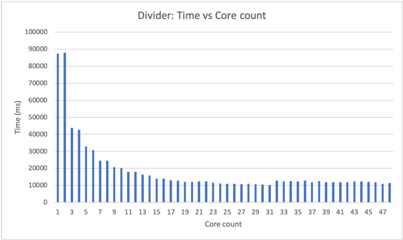
## Bar Chart: Divider: Time vs Core count ### Overview The image displays a vertical bar chart illustrating the relationship between the number of processing cores ("Core count") and the execution time in milliseconds ("Time (ms)") for a computational task labeled "Divider". The chart demonstrates a clear inverse relationship where increasing the core count significantly reduces the execution time, with diminishing returns as the core count becomes high. ### Components/Axes * **Chart Title:** "Divider: Time vs Core count" (positioned at the top center). * **Y-Axis (Vertical):** * **Label:** "Time (ms)" (positioned vertically on the left side). * **Scale:** Linear scale from 0 to 100,000. * **Major Tick Marks:** 0, 10000, 20000, 30000, 40000, 50000, 60000, 70000, 80000, 90000, 100000. * **X-Axis (Horizontal):** * **Label:** "Core count" (positioned at the bottom center). * **Scale:** Linear scale representing discrete core counts. * **Major Tick Mark Labels:** 1, 3, 5, 7, 9, 11, 13, 15, 17, 19, 21, 23, 25, 27, 29, 31, 33, 35, 37, 39, 41, 43, 45, 47. The bars are plotted for every integer core count from 1 to 48. * **Data Series:** A single series represented by blue vertical bars. There is no legend, as only one data category is present. ### Detailed Analysis The chart plots execution time against core count. The trend is a steep, non-linear decline in time as cores are added, which then plateaus. **Trend Verification:** The data series shows a steep downward slope from left (low core count) to right (high core count), which gradually flattens into a near-horizontal line. **Approximate Data Points (Time in ms):** * **Core 1:** ~88,000 ms * **Core 2:** ~88,000 ms (similar to Core 1) * **Core 3:** ~44,000 ms * **Core 4:** ~43,000 ms * **Core 5:** ~33,000 ms * **Core 6:** ~31,000 ms * **Core 7:** ~25,000 ms * **Core 8:** ~24,000 ms * **Core 9:** ~21,000 ms * **Core 10:** ~20,000 ms * **Core 11:** ~18,000 ms * **Core 12:** ~17,000 ms * **Core 13:** ~16,000 ms * **Core 14:** ~15,000 ms * **Core 15:** ~14,000 ms * **Core 16:** ~13,000 ms * **Core 17:** ~12,500 ms * **Core 18:** ~12,000 ms * **Core 19:** ~11,500 ms * **Core 20:** ~11,000 ms * **Core 21:** ~11,000 ms * **Core 22:** ~10,500 ms * **Core 23:** ~10,500 ms * **Core 24:** ~10,000 ms * **Core 25:** ~10,000 ms * **Core 26:** ~10,000 ms * **Core 27:** ~10,000 ms * **Core 28:** ~10,000 ms * **Core 29:** ~10,000 ms * **Core 30:** ~10,000 ms * **Core 31:** ~10,000 ms * **Core 32:** ~12,000 ms (Note: A slight, anomalous increase) * **Core 33:** ~12,000 ms * **Core 34:** ~12,000 ms * **Core 35:** ~12,000 ms * **Core 36:** ~12,000 ms * **Core 37:** ~12,000 ms * **Core 38:** ~12,000 ms * **Core 39:** ~12,000 ms * **Core 40:** ~12,000 ms * **Core 41:** ~12,000 ms * **Core 42:** ~12,000 ms * **Core 43:** ~12,000 ms * **Core 44:** ~12,000 ms * **Core 45:** ~12,000 ms * **Core 46:** ~12,000 ms * **Core 47:** ~12,000 ms * **Core 48:** ~11,000 ms ### Key Observations 1. **Initial Steep Drop:** The most dramatic performance gain occurs when moving from 1-2 cores to 3-4 cores, where time is roughly halved. 2. **Diminishing Returns:** The rate of improvement slows significantly after approximately 16 cores. The curve flattens, indicating that adding more cores yields progressively smaller reductions in execution time. 3. **Performance Plateau:** From approximately core 24 to core 31, the execution time stabilizes around 10,000 ms. 4. **Anomalous Increase:** There is a distinct, small upward jump in execution time at core 32 (to ~12,000 ms), which then remains constant through core 47. This breaks the previous plateau and suggests a potential change in system behavior, resource contention, or measurement artifact at that specific core count. 5. **Final Value:** At the highest plotted core count (48), the time is approximately 11,000 ms, slightly lower than the anomalous plateau but still higher than the minimum observed at cores 24-31. ### Interpretation This chart visualizes the concept of **parallel scaling efficiency** for a specific computational task ("Divider"). The data suggests the task is highly parallelizable initially, as adding cores dramatically reduces runtime. However, it also clearly demonstrates **Amdahl's Law** or the impact of **parallel overhead** (like communication, synchronization, or serial bottlenecks). * **The steep initial decline** indicates that a large portion of the task can be effectively distributed across multiple cores. * **The flattening curve** reveals that beyond a certain point (~16-24 cores), the overhead of managing parallel execution or the remaining serial portion of the code dominates, making additional cores less effective. * **The anomalous increase at core 32** is a critical point for investigation. It could indicate a hardware boundary (e.g., crossing a NUMA node boundary), a software scheduling issue, or a resource conflict (e.g., memory bandwidth saturation) that introduces new inefficiencies at that specific scale. This outlier is more significant than the general trend and would be a key focus for performance optimization. * **The overall takeaway** is that for this "Divider" task, simply maximizing core count is not optimal. There is a "sweet spot" for efficiency (around 24-31 cores in this test), after which performance may degrade or stagnate due to system-level constraints. The chart provides empirical data to guide resource allocation for this specific workload.

## Bar Chart: Divider: Time vs Core count ### Overview The bar chart displays the relationship between the time taken by a divider and the core count. The x-axis represents the core count, ranging from 1 to 47, while the y-axis represents the time in milliseconds, ranging from 0 to 100,000 ms. ### Components/Axes - **Title**: Divider: Time vs Core count - **X-axis**: Core count (ranging from 1 to 47) - **Y-axis**: Time (milliseconds, ranging from 0 to 100,000 ms) - **Legend**: No legend is present in the image. ### Detailed Analysis or ### Content Details The chart shows a clear inverse relationship between the core count and the time taken by the divider. As the core count increases, the time taken decreases. The highest time taken is observed at a core count of 1, with a time of approximately 85,000 ms. The time taken decreases as the core count increases, reaching its lowest point at a core count of 47, with a time of approximately 10,000 ms. ### Key Observations - The highest time taken is at a core count of 1. - The time taken decreases as the core count increases. - The lowest time taken is at a core count of 47. ### Interpretation The data suggests that as the number of cores increases, the time taken by the divider decreases. This could be due to the parallel processing capabilities of multi-core systems, where multiple tasks can be executed simultaneously, reducing the overall time taken. However, it is important to note that the relationship is not linear, as the time taken decreases more rapidly at lower core counts and then levels off at higher core counts. This could be due to the overhead of managing multiple cores and the diminishing returns of additional cores.

## Bar Chart: Divider: Time vs Core count ### Overview The chart visualizes the relationship between core count (x-axis) and processing time in milliseconds (y-axis). It shows a bar graph with 24 vertical blue bars representing time measurements across core counts from 1 to 47. The y-axis scales logarithmically from 0 to 100,000 ms, while the x-axis increments by 2 cores. The title emphasizes a "Divider" relationship between time and core count. ### Components/Axes - **X-axis (Core count)**: Labeled "Core count" with values 1, 3, 5, ..., 47 (odd numbers up to 47). - **Y-axis (Time)**: Labeled "Time (ms)" with logarithmic scale from 0 to 100,000 ms in 10,000 ms increments. - **Legend**: Single blue bar color with no explicit label, implying a single data series. - **Title**: "Divider: Time vs Core count" centered at the top. ### Detailed Analysis - **Core 1**: Tallest bar at ~88,000 ms (highest time). - **Core 3**: ~45,000 ms (50% reduction from Core 1). - **Core 5**: ~32,000 ms (28% reduction from Core 3). - **Core 7**: ~24,000 ms (25% reduction from Core 5). - **Core 9**: ~20,000 ms (20% reduction from Core 7). - **Core 11**: ~18,000 ms (10% reduction from Core 9). - **Cores 13–47**: Bars plateau between ~10,000–12,000 ms, showing minimal variation. ### Key Observations 1. **Steep Initial Decline**: Time drops rapidly from Core 1 to Core 11 (~88,000 ms → ~18,000 ms). 2. **Plateau Effect**: Beyond Core 11, time remains stable (~10,000–12,000 ms) despite doubling core counts. 3. **Diminishing Returns**: Adding cores beyond 11 yields negligible time improvements. 4. **Anomaly**: Core 1’s time (~88,000 ms) is 5.5× higher than Core 3 (~45,000 ms), suggesting non-linear scaling. ### Interpretation The data demonstrates **Amdahl’s Law** in action: parallel processing gains are limited by sequential tasks. The sharp decline up to Core 11 indicates effective parallelization, while the plateau suggests: - **Bottlenecks**: A single-threaded component limiting further optimization. - **Overhead**: Synchronization or communication costs negating benefits of additional cores. - **Hardware Limits**: Physical constraints (e.g., memory bandwidth) capping scalability. The "Divider" title metaphorically represents the threshold (Core 11) where time "divides" into a stable range. This pattern is critical for optimizing parallel workloads, as adding cores beyond 11 offers no practical benefit in this scenario.