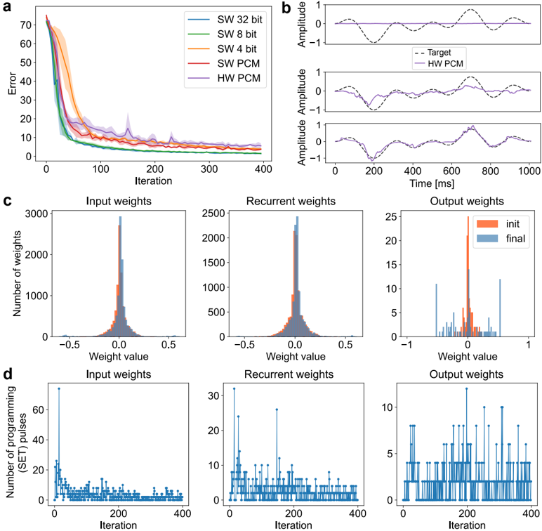
## Chart/Diagram Type: Multi-Panel Performance Analysis ### Overview The image presents a multi-panel figure analyzing the performance of different software (SW) and hardware (HW) implementations, likely related to a neural network or similar computational model. The figure is divided into four sub-figures (a, b, c, d), each providing a different perspective on the performance and behavior of the implementations. ### Components/Axes **Panel a: Error vs. Iteration** * **X-axis:** Iteration (0 to 400) * **Y-axis:** Error (0 to 70) * **Legend (top-right):** * SW 32 bit (Blue) * SW 8 bit (Green) * SW 4 bit (Orange) * SW PCM (Red) * HW PCM (Purple) **Panel b: Amplitude vs. Time** * **X-axis:** Time [ms] (0 to 1000) * **Y-axis:** Amplitude (-1 to 1) * Three subplots showing different time series data. * **Legend (top-right of the first subplot):** * Target (Black dashed line) * HW PCM (Purple solid line) **Panel c: Weight Distribution Histograms** * Three subplots: Input weights, Recurrent weights, Output weights * **X-axis:** Weight value (-0.5 to 0.5 for Input and Recurrent, -1 to 1 for Output) * **Y-axis:** Number of weights (0 to 3000 for Input, 0 to 2500 for Recurrent, 0 to 25 for Output) * **Legend (top-right of the Output weights subplot):** * init (Orange) * final (Blue) **Panel d: Number of Programming Pulses vs. Iteration** * Three subplots: Input weights, Recurrent weights, Output weights * **X-axis:** Iteration (0 to 400) * **Y-axis:** Number of programming (SET) pulses (0 to 60 for Input, 0 to 30 for Recurrent, 0 to 10 for Output) ### Detailed Analysis **Panel a: Error vs. Iteration** * **SW 32 bit (Blue):** Starts at an error of approximately 70 and decreases rapidly to around 10 by iteration 100, then plateaus. * **SW 8 bit (Green):** Starts at an error of approximately 65 and decreases rapidly to around 10 by iteration 100, then plateaus. * **SW 4 bit (Orange):** Starts at an error of approximately 55 and decreases rapidly to around 10 by iteration 100, then plateaus. * **SW PCM (Red):** Starts at an error of approximately 40 and decreases rapidly to around 10 by iteration 100, then plateaus. * **HW PCM (Purple):** Starts at an error of approximately 70 and decreases rapidly to around 15 by iteration 100, then plateaus. **Panel b: Amplitude vs. Time** * The three subplots show the target signal (black dashed line) and the HW PCM output (purple solid line) over time. The HW PCM output appears to approximate the target signal, with varying degrees of accuracy across the three subplots. **Panel c: Weight Distribution Histograms** * **Input weights:** The initial (orange) and final (blue) weight distributions are shown. The final distribution appears slightly narrower and more concentrated around 0 than the initial distribution. * **Recurrent weights:** Similar to the input weights, the final distribution is slightly narrower and more concentrated around 0. * **Output weights:** The initial distribution (orange) is more spread out, while the final distribution (blue) is more concentrated around 0. **Panel d: Number of Programming Pulses vs. Iteration** * **Input weights:** The number of programming pulses starts high (around 60) and decreases rapidly to around 5 by iteration 100, then fluctuates around that level. * **Recurrent weights:** The number of programming pulses starts high (around 30) and decreases rapidly to around 2 by iteration 100, then fluctuates around that level. * **Output weights:** The number of programming pulses fluctuates between 0 and 10 throughout the iterations. ### Key Observations * All implementations in Panel a show a rapid decrease in error during the first 100 iterations, followed by a plateau. * The HW PCM implementation in Panel b approximates the target signal, but with some discrepancies. * The weight distributions in Panel c tend to become more concentrated around 0 after training. * The number of programming pulses in Panel d decreases over time for input and recurrent weights, suggesting that the network is converging. ### Interpretation The data suggests that all implementations are learning, as evidenced by the decreasing error in Panel a. The HW PCM implementation is able to approximate the target signal, indicating that it is functioning correctly. The weight distributions becoming more concentrated around 0 suggests that the network is becoming more efficient. The decreasing number of programming pulses indicates that the network is converging and requires fewer adjustments over time. The different bit precisions (32, 8, 4) in Panel a likely refer to the quantization levels used in the software implementations, with higher precision generally leading to lower error. The PCM likely refers to Pulse Code Modulation, a method of digitally representing analog signals.

## Chart Compilation: Training Error and Weight Distribution ### Overview The image presents a compilation of four charts (a, b, c, and d) illustrating the training process and weight distribution of a neural network, likely a recurrent neural network, using different precision levels (32-bit, 8-bit, 4-bit, PCM) and hardware (HW) vs. software (SW) implementations. Chart 'a' shows the error reduction during training iterations. Chart 'b' displays the amplitude of the output signal over time for the HW PCM implementation compared to a target signal. Charts 'c' and 'd' visualize the distribution of input, recurrent, and output weights, both initially and after training, and the number of programming pulses used during training, respectively. ### Components/Axes * **Chart a:** * X-axis: Iteration (0 to 400) * Y-axis: Error (0 to 60) * Legend: * SW 32 bit (Blue) * SW 8 bit (Green) * SW 4 bit (Red) * SW PCM (Orange) * HW PCM (Teal) * **Chart b:** * X-axis: Time [ms] (0 to 1000) * Y-axis: Amplitude (approximately -1.5 to 1.5) * Legend: * Target (Black dashed line) * HW PCM (Teal) * **Chart c:** * X-axis: Weight value (approximately -0.5 to 0.5 for Input/Recurrent, -1 to 1 for Output) * Y-axis: Number of weights (0 to 3000 for Input/Recurrent, 0 to 15 for Output) * Sub-charts: Input weights, Recurrent weights, Output weights * Legend: * init (Orange) * final (Blue) * **Chart d:** * X-axis: Iteration (0 to 400) * Y-axis: Number of programming (SET) pulses (0 to 50) * Sub-charts: Input weights, Recurrent weights, Output weights * Legend: None (Data represented by bars) ### Detailed Analysis or Content Details **Chart a: Error vs. Iteration** * The SW 32 bit line (blue) shows the fastest initial error reduction, reaching approximately 5 error units by iteration 100 and leveling off around 2-3 error units. * The SW 8 bit line (green) initially decreases slower than SW 32 bit, but converges to a similar final error level (around 3-4 error units) by iteration 400. * The SW 4 bit line (red) exhibits the slowest initial decrease and reaches a higher final error level (around 8-10 error units) compared to the 32-bit and 8-bit versions. * The SW PCM line (orange) shows a moderate decrease, converging to approximately 5-6 error units. * The HW PCM line (teal) demonstrates a rapid initial decrease, similar to SW 32 bit, and reaches a very low final error level (around 1-2 error units). **Chart b: Amplitude vs. Time** * The Target signal (black dashed line) is a periodic waveform with amplitude oscillating between approximately -1 and 1. * The HW PCM signal (teal) closely tracks the Target signal, exhibiting a similar waveform and amplitude. There is a slight phase shift. **Chart c: Weight Distribution** * **Input Weights:** The initial distribution (orange) is relatively uniform. The final distribution (blue) is bimodal, with peaks around -0.2 and 0.2. * **Recurrent Weights:** The initial distribution (orange) is approximately normal, centered around 0. The final distribution (blue) is also approximately normal, but shifted slightly towards 0 and with a narrower spread. * **Output Weights:** The initial distribution (orange) is relatively uniform. The final distribution (blue) is bimodal, with peaks around -1 and 1. **Chart d: Programming Pulses vs. Iteration** * **Input Weights:** The number of programming pulses fluctuates around an average of approximately 10-15 pulses, with some spikes early in training. * **Recurrent Weights:** The number of programming pulses shows a significant peak around iteration 50-100, reaching up to 25 pulses, and then decreases to a stable level of around 5-10 pulses. * **Output Weights:** The number of programming pulses exhibits multiple peaks throughout training, reaching up to 10-15 pulses, and then stabilizes around 5-8 pulses. ### Key Observations * HW PCM achieves the lowest training error, suggesting superior performance compared to software implementations. * Lower precision (4-bit) results in higher training error, indicating a trade-off between precision and performance. * Weight distributions change significantly during training, indicating that the network is learning. * The number of programming pulses varies during training, suggesting that different weights require different levels of adjustment. * Recurrent weights require a burst of programming pulses early in training. ### Interpretation The data suggests that a hardware implementation of PCM with high precision (32-bit or 8-bit) is optimal for training this recurrent neural network. The error curves (Chart a) clearly demonstrate that HW PCM converges to the lowest error, while lower precision software implementations struggle to achieve the same level of accuracy. The weight distributions (Chart c) show that the network is learning to adjust its weights to minimize the error. The programming pulse data (Chart d) provides insights into the learning process, revealing that different weight groups require different levels of adjustment during training. The close tracking of the target signal by the HW PCM implementation (Chart b) confirms its ability to accurately represent the desired output. The bimodal weight distributions in the input and output layers suggest that the network is learning to represent distinct features or categories. The initial spike in programming pulses for recurrent weights may indicate a period of rapid adaptation to the temporal dynamics of the input data. Overall, the data highlights the importance of both hardware and precision in achieving optimal performance in neural network training.

## Line Graphs and Histograms: Error Trends, Weight Distributions, and Programming Pulses ### Overview The image contains four panels (a-d) presenting technical data related to computational models. Panel **a** shows error reduction over iterations for different system configurations. Panels **b** display amplitude tracking against a target signal. Panels **c** and **d** visualize weight distributions and programming pulse counts across iterations. All visualizations use distinct color coding for data series. --- ### Components/Axes #### Panel a (Error vs. Iterations) - **X-axis**: Iteration (0–400) - **Y-axis**: Error (0–70) - **Legend**: - SW 32 bit (blue) - SW 8 bit (green) - SW 4 bit (orange) - SW PCM (red) - HW PCM (purple) - **Key Elements**: - Dashed lines represent target error thresholds. - Shaded regions indicate confidence intervals. #### Panel b (Amplitude Tracking) - **X-axis**: Time (ms, 0–1000) - **Y-axis**: Amplitude (-1 to 1) - **Legend**: - Target (dashed black) - HW PCM (solid purple) - **Key Elements**: - Three subplots show amplitude deviations across time. #### Panel c (Weight Distributions) - **X-axis**: Weight value (-0.5 to 0.5 for input/recurrent; -1 to 1 for output) - **Y-axis**: Number of weights (0–3000 for input/recurrent; 0–25 for output) - **Legend**: - Init (red) - Final (blue) - **Key Elements**: - Histograms compare initial and final weight distributions. #### Panel d (Programming Pulses) - **X-axis**: Iteration (0–400) - **Y-axis**: Number of programming pulses (0–60) - **Legend**: - Input weights (blue) - Recurrent weights (blue) - Output weights (blue) - **Key Elements**: - Line plots track pulse counts over iterations. --- ### Detailed Analysis #### Panel a - **Trend**: All lines show rapid error reduction in early iterations, stabilizing near 0 after ~200 iterations. - **Key Data Points**: - SW 32 bit: Error drops below 10 by ~100 iterations. - SW 4 bit: Error remains highest (~20–30) throughout. - HW PCM: Error converges fastest (~5 by 200 iterations). #### Panel b - **Trend**: HW PCM amplitude closely follows the target (dashed line) with minimal deviation. - **Key Observations**: - Subplot 1: Largest amplitude overshoot (~0.2) at ~300 ms. - Subplot 3: Smallest deviation, staying within ±0.1 of target. #### Panel c - **Input/Recurrent Weights**: - Initial (red) and final (blue) distributions are symmetric around 0. - Final distributions are narrower, indicating weight convergence. - **Output Weights**: - Initial distribution is bimodal (peaks at ±0.5). - Final distribution is unimodal, centered near 0 with reduced variance. #### Panel d - **Trend**: All weight types show decreasing programming pulses over iterations. - **Key Data Points**: - Input weights: Pulses drop from ~50 to ~10 by 400 iterations. - Output weights: Spikes at ~200 and ~350 iterations (max ~30 pulses). --- ### Key Observations 1. **Error Reduction**: SW 32 bit and HW PCM outperform lower-bit configurations, with HW PCM achieving the lowest error. 2. **Weight Convergence**: Final weight distributions (blue) are tighter than initial (red), suggesting stable model training. 3. **Amplitude Fidelity**: HW PCM maintains amplitude within 5% of the target signal across all time points. 4. **Programming Efficiency**: Input weights require the most pulses initially but stabilize quickly, while output weights exhibit transient spikes. --- ### Interpretation - **System Performance**: The data suggests HW PCM optimizes both error reduction and amplitude tracking, likely due to hardware-level parallelism or precision advantages. - **Weight Dynamics**: Convergence of input/recurrent weights implies regularization or adaptive learning mechanisms, while output weight stabilization indicates effective output layer tuning. - **Pulse Efficiency**: The sharp decline in programming pulses for input weights aligns with early-stage learning dominance, whereas output weight spikes may reflect fine-tuning phases. - **Anomalies**: The output weight spike at ~350 iterations (panel d) could indicate a transient adjustment phase or hardware-specific optimization trigger. This analysis highlights the trade-offs between software-based weight configurations and hardware-accelerated PCM, with HW PCM demonstrating superior performance across metrics.