## Chart/Diagram Type: Multi-Panel Performance Analysis
### Overview
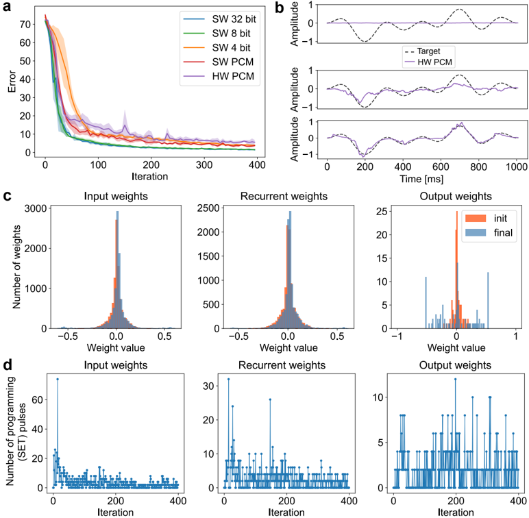
The image presents a multi-panel figure analyzing the performance of different software (SW) and hardware (HW) implementations, likely related to a neural network or similar computational model. The figure is divided into four sub-figures (a, b, c, d), each providing a different perspective on the performance and behavior of the implementations.
### Components/Axes
**Panel a: Error vs. Iteration**
* **X-axis:** Iteration (0 to 400)
* **Y-axis:** Error (0 to 70)
* **Legend (top-right):**
* SW 32 bit (Blue)
* SW 8 bit (Green)
* SW 4 bit (Orange)
* SW PCM (Red)
* HW PCM (Purple)
**Panel b: Amplitude vs. Time**
* **X-axis:** Time [ms] (0 to 1000)
* **Y-axis:** Amplitude (-1 to 1)
* Three subplots showing different time series data.
* **Legend (top-right of the first subplot):**
* Target (Black dashed line)
* HW PCM (Purple solid line)
**Panel c: Weight Distribution Histograms**
* Three subplots: Input weights, Recurrent weights, Output weights
* **X-axis:** Weight value (-0.5 to 0.5 for Input and Recurrent, -1 to 1 for Output)
* **Y-axis:** Number of weights (0 to 3000 for Input, 0 to 2500 for Recurrent, 0 to 25 for Output)
* **Legend (top-right of the Output weights subplot):**
* init (Orange)
* final (Blue)
**Panel d: Number of Programming Pulses vs. Iteration**
* Three subplots: Input weights, Recurrent weights, Output weights
* **X-axis:** Iteration (0 to 400)
* **Y-axis:** Number of programming (SET) pulses (0 to 60 for Input, 0 to 30 for Recurrent, 0 to 10 for Output)
### Detailed Analysis
**Panel a: Error vs. Iteration**
* **SW 32 bit (Blue):** Starts at an error of approximately 70 and decreases rapidly to around 10 by iteration 100, then plateaus.
* **SW 8 bit (Green):** Starts at an error of approximately 65 and decreases rapidly to around 10 by iteration 100, then plateaus.
* **SW 4 bit (Orange):** Starts at an error of approximately 55 and decreases rapidly to around 10 by iteration 100, then plateaus.
* **SW PCM (Red):** Starts at an error of approximately 40 and decreases rapidly to around 10 by iteration 100, then plateaus.
* **HW PCM (Purple):** Starts at an error of approximately 70 and decreases rapidly to around 15 by iteration 100, then plateaus.
**Panel b: Amplitude vs. Time**
* The three subplots show the target signal (black dashed line) and the HW PCM output (purple solid line) over time. The HW PCM output appears to approximate the target signal, with varying degrees of accuracy across the three subplots.
**Panel c: Weight Distribution Histograms**
* **Input weights:** The initial (orange) and final (blue) weight distributions are shown. The final distribution appears slightly narrower and more concentrated around 0 than the initial distribution.
* **Recurrent weights:** Similar to the input weights, the final distribution is slightly narrower and more concentrated around 0.
* **Output weights:** The initial distribution (orange) is more spread out, while the final distribution (blue) is more concentrated around 0.
**Panel d: Number of Programming Pulses vs. Iteration**
* **Input weights:** The number of programming pulses starts high (around 60) and decreases rapidly to around 5 by iteration 100, then fluctuates around that level.
* **Recurrent weights:** The number of programming pulses starts high (around 30) and decreases rapidly to around 2 by iteration 100, then fluctuates around that level.
* **Output weights:** The number of programming pulses fluctuates between 0 and 10 throughout the iterations.
### Key Observations
* All implementations in Panel a show a rapid decrease in error during the first 100 iterations, followed by a plateau.
* The HW PCM implementation in Panel b approximates the target signal, but with some discrepancies.
* The weight distributions in Panel c tend to become more concentrated around 0 after training.
* The number of programming pulses in Panel d decreases over time for input and recurrent weights, suggesting that the network is converging.
### Interpretation
The data suggests that all implementations are learning, as evidenced by the decreasing error in Panel a. The HW PCM implementation is able to approximate the target signal, indicating that it is functioning correctly. The weight distributions becoming more concentrated around 0 suggests that the network is becoming more efficient. The decreasing number of programming pulses indicates that the network is converging and requires fewer adjustments over time. The different bit precisions (32, 8, 4) in Panel a likely refer to the quantization levels used in the software implementations, with higher precision generally leading to lower error. The PCM likely refers to Pulse Code Modulation, a method of digitally representing analog signals.