## [Dual-Panel Chart]: Training Loss and Local Learning Coefficient vs. Iteration
### Overview
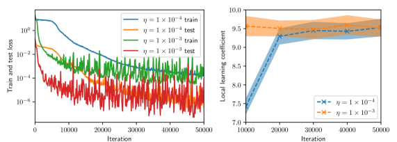
The image contains two side-by-side line charts. The left chart plots training and test loss on a logarithmic scale against training iterations for two different learning rates (η). The right chart plots the "Local learning coefficient" against iterations for the same two learning rates, with shaded regions indicating variance or confidence intervals. The overall purpose is to compare the training dynamics and a derived metric (local learning coefficient) for two different hyperparameter settings.
### Components/Axes
**Left Chart:**
* **Chart Type:** Line chart with logarithmic y-axis.
* **X-axis:** Label: "Iteration". Scale: Linear, from 0 to 50,000, with major ticks at 0, 10000, 20000, 30000, 40000, 50000.
* **Y-axis:** Label: "Train and test loss". Scale: Logarithmic (base 10), from 10^-6 to 10^0 (1).
* **Legend:** Located in the top-right corner of the plot area. Contains four entries:
1. Blue solid line: `η = 1 × 10⁻⁴ train`
2. Orange dashed line: `η = 1 × 10⁻⁴ test`
3. Green solid line: `η = 1 × 10⁻³ train`
4. Red dashed line: `η = 1 × 10⁻³ test`
**Right Chart:**
* **Chart Type:** Line chart with shaded confidence/variance bands.
* **X-axis:** Label: "Iteration". Scale: Linear, from 10,000 to 50,000, with major ticks at 10000, 20000, 30000, 40000, 50000.
* **Y-axis:** Label: "Local learning coefficient". Scale: Linear, from 7.0 to 10.0, with major ticks at 7.0, 7.5, 8.0, 8.5, 9.0, 9.5, 10.0.
* **Legend:** Located in the bottom-right corner of the plot area. Contains two entries:
1. Blue line with 'x' markers and blue shaded band: `η = 1 × 10⁻⁴`
2. Orange line with 'x' markers and orange shaded band: `η = 1 × 10⁻³`
### Detailed Analysis
**Left Chart - Loss vs. Iteration:**
* **Trend Verification:** All four series show a general downward trend, indicating decreasing loss as training progresses. The lines for the higher learning rate (η=1×10⁻³, green/red) are consistently lower on the y-axis than those for the lower learning rate (η=1×10⁻⁴, blue/orange).
* **Data Series & Approximate Values:**
* **η = 1 × 10⁻⁴ train (Blue solid):** Starts near 10^0 (1.0) at iteration 0. Decreases steadily, crossing 10^-1 (~0.1) around iteration 10,000, and 10^-2 (~0.01) around iteration 25,000. Ends near 10^-3 (~0.001) at iteration 50,000.
* **η = 1 × 10⁻⁴ test (Orange dashed):** Follows a similar but noisier path to its training counterpart. Starts near 10^0, shows significant variance, and ends in the range of 10^-3 to 10^-2.
* **η = 1 × 10⁻³ train (Green solid):** Starts lower, around 10^-1 (~0.1) at iteration 0. Decreases rapidly, reaching 10^-3 (~0.001) by iteration 10,000. Continues to decrease with high-frequency noise, ending near 10^-4 (~0.0001) at iteration 50,000.
* **η = 1 × 10⁻³ test (Red dashed):** Follows the green training line closely but with even greater noise/fluctuation. Its final value at 50,000 iterations is approximately between 10^-5 and 10^-4.
**Right Chart - Local Learning Coefficient vs. Iteration:**
* **Trend Verification:** Both series show an upward trend, indicating the local learning coefficient increases with training iterations. The series for η=1×10⁻³ (orange) is consistently above the series for η=1×10⁻⁴ (blue).
* **Data Series & Approximate Values:**
* **η = 1 × 10⁻⁴ (Blue):** At iteration 10,000, the value is approximately 7.3. It rises sharply to about 9.3 by iteration 20,000. The increase slows, reaching approximately 9.4 by iteration 50,000. The blue shaded band (variance) is narrow, spanning roughly ±0.2 around the line.
* **η = 1 × 10⁻³ (Orange):** At iteration 10,000, the value is already high, approximately 9.5. It increases gradually and relatively linearly, reaching approximately 9.7 by iteration 50,000. The orange shaded band is wider than the blue one, especially at later iterations, spanning roughly ±0.3 to ±0.4 around the line.
### Key Observations
1. **Learning Rate Impact:** The higher learning rate (η=1×10⁻³) leads to significantly lower loss values (by 1-2 orders of magnitude) throughout training compared to the lower rate (η=1×10⁻⁴).
2. **Loss Noise:** Test loss curves (dashed lines) are substantially noisier than their corresponding training loss curves (solid lines), which is typical.
3. **Coefficient Convergence:** The local learning coefficient for the lower learning rate (blue) shows a period of rapid increase between 10k and 20k iterations before plateauing. The coefficient for the higher learning rate (orange) starts high and increases slowly, suggesting it may be in a different phase of learning.
4. **Variance:** The shaded bands on the right chart indicate greater variance/uncertainty in the local learning coefficient estimate for the higher learning rate (η=1×10⁻³).
### Interpretation
This data suggests a trade-off or different dynamic governed by the learning rate hyperparameter (η). The higher learning rate (1×10⁻³) achieves a much lower loss faster, indicating more aggressive optimization. However, its associated "local learning coefficient" is higher and more variable, which might imply the optimization is occurring in a region of the loss landscape with different curvature properties or that the parameter updates are more stochastic.
The lower learning rate (1×10⁻⁴) results in higher loss but a learning coefficient that evolves from a low value to a stable plateau. This could indicate a more gradual, stable descent into a minimum. The fact that the coefficient for the higher learning rate is always above that of the lower one, even when loss is lower, is a key finding. It suggests the local learning coefficient is not a simple proxy for loss but captures a distinct property of the training dynamics, possibly related to the effective step size or the geometry of the optimization path. The investigation appears to be probing the relationship between a hyperparameter, the resulting loss, and a derived metric that may offer deeper insight into the learning process.