\n
## Mathematical Plot: Conditional Probability Density Functions
### Overview
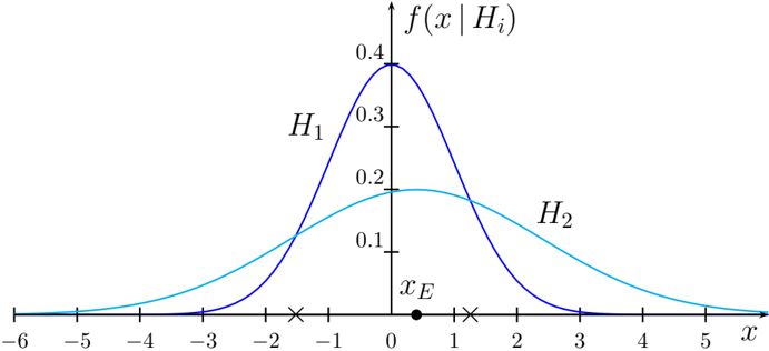
The image displays a mathematical plot comparing two conditional probability density functions (PDFs), labeled \(H_1\) and \(H_2\), plotted against a variable \(x\). The plot illustrates how the probability density of an observation \(x\) differs under two distinct hypotheses or conditions, \(H_1\) and \(H_2\). A specific point on the x-axis, labeled \(x_E\), is marked, likely representing an observed evidence value.
### Components/Axes
* **Vertical Axis (Y-axis):** Labeled \(f(x|H_i)\), representing the conditional probability density function of \(x\) given hypothesis \(H_i\). The axis has numerical tick marks at intervals of 0.1, ranging from 0.0 to 0.4.
* **Horizontal Axis (X-axis):** Labeled \(x\). The axis has numerical tick marks at integer intervals from -6 to 5. There are additional non-numeric markers: an 'x' at approximately \(x = -1.5\), a solid dot labeled \(x_E\) at approximately \(x = 0.5\), and another 'x' at approximately \(x = 1.5\).
* **Data Series (Curves):**
* **Curve \(H_1\):** A dark blue, bell-shaped curve. It is taller and narrower.
* **Curve \(H_2\):** A cyan (light blue), bell-shaped curve. It is shorter and wider.
* **Labels:**
* \(H_1\): Positioned in the upper-left quadrant, near the peak of the dark blue curve.
* \(H_2\): Positioned in the upper-right quadrant, on the descending slope of the cyan curve.
* \(x_E\): Positioned directly above a solid black dot on the x-axis, between 0 and 1.
* \(f(x|H_i)\): Positioned at the top of the y-axis, serving as the overall title for the vertical axis.
### Detailed Analysis
* **Curve \(H_1\) (Dark Blue):**
* **Trend:** The curve rises steeply from the left, peaks sharply, and then descends steeply. It is symmetric around its peak.
* **Key Points (Approximate):**
* Peak Location: \(x \approx 0\).
* Peak Value: \(f(x|H_1) \approx 0.4\).
* The curve approaches near-zero density around \(x = -3\) and \(x = 3\).
* **Curve \(H_2\) (Cyan):**
* **Trend:** The curve rises more gradually, has a broader, flatter peak, and descends more gradually. It is also symmetric.
* **Key Points (Approximate):**
* Peak Location: \(x \approx 1\).
* Peak Value: \(f(x|H_2) \approx 0.18\).
* The curve approaches near-zero density around \(x = -5\) and \(x = 5\).
* **Intersection:** The two curves intersect at two points. One intersection is near \(x = -1.5\) (marked with an 'x'), and the other is near \(x = 1.5\) (marked with an 'x').
* **Evidence Point \(x_E\):** A specific value \(x_E \approx 0.5\) is marked with a solid dot on the x-axis. At this point, the density value for \(H_1\) is higher than for \(H_2\).
### Key Observations
1. **Distribution Characteristics:** \(H_1\) represents a distribution with a smaller variance (more concentrated around its mean of ~0), while \(H_2\) represents a distribution with a larger variance (more spread out around its mean of ~1).
2. **Likelihood Ratio:** For any given \(x\), the ratio \(f(x|H_1) / f(x|H_2)\) indicates the relative likelihood of observing \(x\) under \(H_1\) versus \(H_2\). This ratio is greater than 1 for \(x\) values between the two intersection points (approximately -1.5 to 1.5), favoring \(H_1\). Outside this range, the ratio is less than 1, favoring \(H_2\).
3. **Evidence Interpretation:** The marked point \(x_E \approx 0.5\) falls within the region where \(H_1\) has a higher density. This suggests that the observed evidence \(x_E\) is more probable under hypothesis \(H_1\) than under \(H_2\).
### Interpretation
This plot is a classic visualization used in statistical hypothesis testing, decision theory, or Bayesian inference. It demonstrates the concept of **likelihood**. The two curves represent the probability distributions of a test statistic or observable data under two competing hypotheses.
* **The Core Idea:** The plot shows how an observed data point (\(x_E\)) can be used to compare hypotheses. The hypothesis under which the observed data is more likely (has a higher probability density) is often considered the better explanation for that data.
* **Trade-off Between Bias and Variance:** In a machine learning context, this could illustrate the bias-variance tradeoff. \(H_1\) (low variance, potentially high bias) and \(H_2\) (high variance, potentially low bias) could represent two models. The plot shows their predictive distributions. The optimal model choice depends on where the true data-generating distribution lies.
* **Decision Boundary:** The intersection points (marked with 'x') define the **decision boundaries**. If one were to classify an observation \(x\) based on which hypothesis is more likely, the rule would be: choose \(H_1\) if \(x\) is between the boundaries, and choose \(H_2\) otherwise. The point \(x_E\) would lead to choosing \(H_1\).
* **The Role of \(x_E\):** This point acts as a concrete example. It visually answers the question: "Given this specific observation, which hypothesis is more supported?" The plot makes it clear that \(x_E\) is in a region where the dark blue curve (\(H_1\)) is above the cyan curve (\(H_2\)), providing visual evidence in favor of \(H_1\).
In summary, the image is a technical diagram illustrating the fundamental statistical principle of comparing probability distributions to evaluate evidence for competing explanations.