## Density Plot: Positive vs. Negative Samples
### Overview
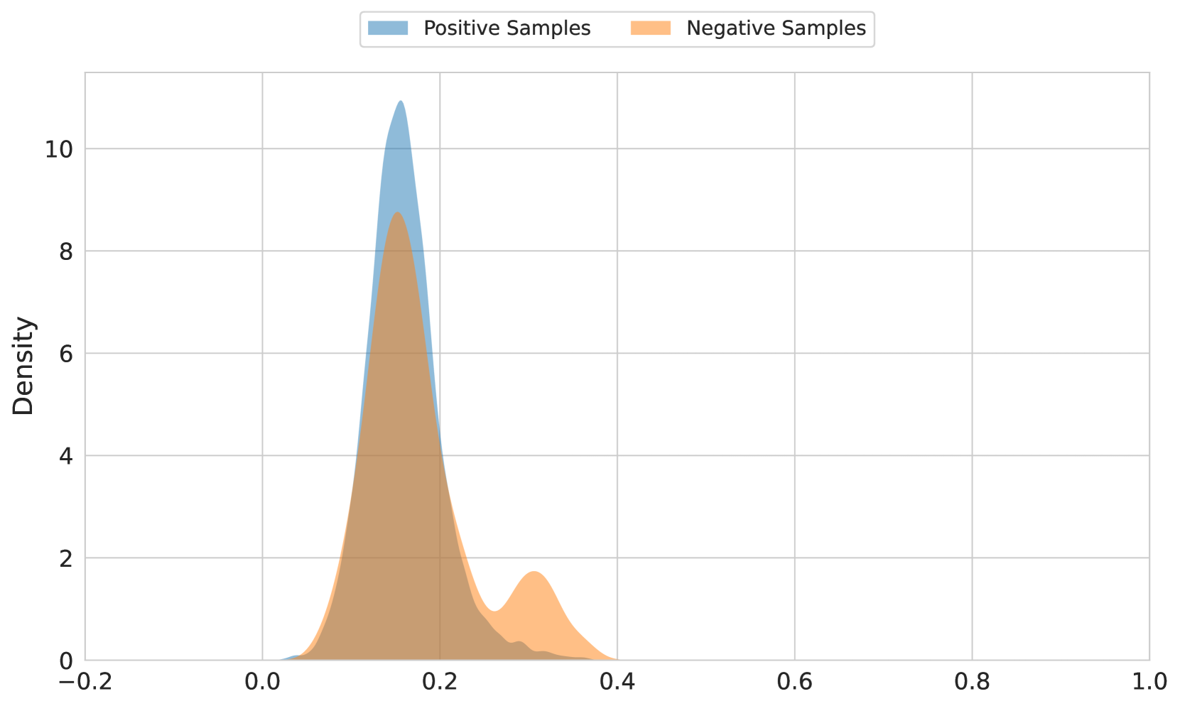
The image is a density plot comparing the distribution of "Positive Samples" and "Negative Samples." The x-axis represents an unspecified variable ranging from approximately -0.2 to 1.0, while the y-axis represents density, ranging from 0 to 10. The plot shows the probability density of each sample type across the range of the x-axis.
### Components/Axes
* **X-axis:** Ranges from -0.2 to 1.0, with tick marks at -0.2, 0.0, 0.2, 0.4, 0.6, 0.8, and 1.0. The x-axis label is not explicitly provided in the image.
* **Y-axis:** Labeled "Density," ranging from 0 to 10, with tick marks at 2, 4, 6, 8, and 10.
* **Legend:** Located at the top of the chart.
* "Positive Samples" is represented by a light blue filled curve.
* "Negative Samples" is represented by a light orange filled curve.
### Detailed Analysis
* **Positive Samples (Light Blue):**
* The density curve for positive samples peaks sharply around x = 0.15, reaching a density of approximately 10.8.
* The curve rapidly decreases after the peak, approaching zero density around x = 0.4.
* The curve remains near zero for x values greater than 0.4.
* **Negative Samples (Light Orange):**
* The density curve for negative samples has two peaks. The primary peak is around x = 0.17, reaching a density of approximately 8.8.
* A secondary, smaller peak occurs around x = 0.35, reaching a density of approximately 1.8.
* The curve approaches zero density around x = 0.6.
### Key Observations
* Both positive and negative samples have their highest density around x = 0.15-0.17.
* The positive samples have a higher peak density than the negative samples at their primary peak.
* The negative samples exhibit a secondary peak around x = 0.35, which is not present in the positive samples distribution.
* Both distributions are skewed to the right.
### Interpretation
The density plot suggests that both positive and negative samples are concentrated around a similar value (approximately 0.15-0.17). However, the presence of a secondary peak in the negative samples distribution indicates that there is a subset of negative samples with a higher value (around 0.35) that is not present in the positive samples. This difference in distribution could be significant depending on what these samples represent. The higher peak density of positive samples at the primary peak suggests that the variable being measured is more strongly associated with positive samples than negative samples at that value.