TECHNICAL ASSET FINGERPRINT
2cec93ce84e962ea35c47a6b
Click to view fullscreen
Press ESC or click to close
FOUND IN PAPERS
EXPERT: healer-alpha-free VERSION 1
RUNTIME: free/openrouter/healer-alpha
INTEL_VERIFIED
## Diagram: Parallel Processor Data Flow Over Time
### Overview
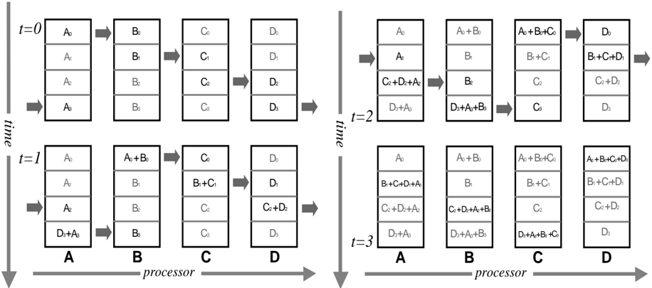
The image is a technical diagram illustrating the flow and combination of data elements across four processors (A, B, C, D) over four discrete time steps (t=0, t=1, t=2, t=3). It visually represents a parallel computing or data processing pipeline where data is passed between processors and aggregated over time.
### Components/Axes
* **Time Axis:** A vertical arrow on the left side of each panel labeled "time" points downward, indicating the progression from t=0 to t=3.
* **Processor Axis:** A horizontal arrow at the bottom of each panel labeled "processor" points to the right, indicating the sequence from processor A to D.
* **Processors:** Four vertical columns in each panel, labeled **A**, **B**, **C**, and **D** at the bottom.
* **Data Elements:** Represented as text within rectangular boxes stacked vertically inside each processor column. Elements are labeled with a letter and subscript (e.g., `A₀`, `B₁`).
* **Data Flow:** Indicated by gray arrows pointing from the output of one processor to the input of the next processor to its right.
* **Panels:** The diagram is split into four main panels, each corresponding to a specific time step:
* Top-left panel: `t=0`
* Bottom-left panel: `t=1`
* Top-right panel: `t=2`
* Bottom-right panel: `t=3`
### Detailed Analysis
The diagram shows how data elements are processed and combined sequentially across processors A→B→C→D at each time step. The state of each processor's data stack evolves over time.
**Time Step t=0 (Top-Left Panel):**
* **Processor A:** Contains four independent data elements: `A₀`, `A₁`, `A₂`, `A₃`.
* **Flow A→B:** An arrow indicates data moves from A to B.
* **Processor B:** Contains four independent data elements: `B₀`, `B₁`, `B₂`, `B₃`.
* **Flow B→C:** An arrow indicates data moves from B to C.
* **Processor C:** Contains four independent data elements: `C₀`, `C₁`, `C₂`, `C₃`.
* **Flow C→D:** An arrow indicates data moves from C to D.
* **Processor D:** Contains four independent data elements: `D₀`, `D₁`, `D₂`, `D₃`.
**Time Step t=1 (Bottom-Left Panel):**
* **Processor A:** Contains `A₀`, `A₁`, `A₂`, and a combined element `D₃+A₀` at the bottom.
* **Flow A→B:** An arrow indicates data moves from A to B.
* **Processor B:** The top element is now a combination `A₀+B₀`. Below are `B₁`, `B₂`, `B₃`.
* **Flow B→C:** An arrow indicates data moves from B to C.
* **Processor C:** The second element is now a combination `B₁+C₁`. The stack is `C₀`, `B₁+C₁`, `C₂`, `C₃`.
* **Flow C→D:** An arrow indicates data moves from C to D.
* **Processor D:** The third element is now a combination `C₂+D₂`. The stack is `D₀`, `D₁`, `C₂+D₂`, `D₃`.
**Time Step t=2 (Top-Right Panel):**
* **Processor A:** The stack is `A₀`, `A₁`, `C₂+D₂+A₂`, `D₃+A₃`.
* **Flow A→B:** An arrow indicates data moves from A to B.
* **Processor B:** The top element is `A₀+B₀`. The third element is `B₂`. The bottom element is `D₃+A₃+B₃`.
* **Flow B→C:** An arrow indicates data moves from B to C.
* **Processor C:** The top element is `A₀+B₀+C₀`. The second element is `B₁+C₁`. The stack is `A₀+B₀+C₀`, `B₁+C₁`, `C₂`, `C₃`.
* **Flow C→D:** An arrow indicates data moves from C to D.
* **Processor D:** The top element is `D₀`. The second element is `B₁+C₁+D₁`. The third element is `C₂+D₂`. The bottom element is `D₃`.
**Time Step t=3 (Bottom-Right Panel):**
* **Processor A:** The stack is `A₀`, `B₁+C₁+D₁+A₁`, `C₂+D₂+A₂`, `D₃+A₃`.
* **Flow A→B:** An arrow indicates data moves from A to B.
* **Processor B:** The top element is `A₀+B₀`. The second element is `B₁`. The third element is `C₂+D₂+A₂+B₂`. The bottom element is `D₃+A₃+B₃`.
* **Flow B→C:** An arrow indicates data moves from B to C.
* **Processor C:** The top element is `A₀+B₀+C₀`. The second element is `B₁+C₁`. The third element is `C₂`. The bottom element is `D₃+A₃+B₃+C₃`.
* **Flow C→D:** An arrow indicates data moves from C to D.
* **Processor D:** The top element is `A₀+B₀+C₀+D₀`. The second element is `B₁+C₁+D₁`. The third element is `C₂+D₂`. The bottom element is `D₃`.
### Key Observations
1. **Accumulation Pattern:** Data elements become increasingly combined as time progresses. By t=3, the top element of Processor D is the sum of all initial '0' subscript elements (`A₀+B₀+C₀+D₀`).
2. **Asynchronous Combination:** Combinations do not happen uniformly. For example, at t=1, Processor B combines `A₀+B₀`, while Processor C combines `B₁+C₁`, and Processor D combines `C₂+D₂`. This suggests a staggered or pipelined reduction operation.
3. **Data Persistence:** Original data elements (e.g., `A₀`, `B₁`) often remain visible in the stacks even after being used in a combination, indicating they might be copied rather than moved.
4. **Flow Direction:** The gray arrows consistently show a left-to-right data flow (A→B→C→D) within each time step, but the vertical "time" axis shows the entire system state evolving downward.
5. **Spatial Layout:** The four time-step panels are arranged in a 2x2 grid. The `t=0` and `t=1` panels are on the left, stacked vertically. The `t=2` and `t=3` panels are on the right, also stacked vertically.
### Interpretation
This diagram likely models a **parallel prefix sum (scan) operation** or a similar **parallel reduction algorithm** across a linear array of processors. The goal is to compute a cumulative result (e.g., a sum) for all data elements.
* **What it demonstrates:** It shows how a global operation can be broken down into local communication and computation steps. Each processor performs a partial combination and passes results downstream. The staggered combinations (`A₀+B₀` at t=1, then `A₀+B₀+C₀` at t=2, then `A₀+B₀+C₀+D₀` at t=3) are characteristic of a **recursive doubling** or **pipeline** approach to prefix computation.
* **Relationship between elements:** Processors are interdependent. The output of Processor A at time `t` becomes an input for Processor B at time `t+1` (or the same time step, depending on the model). The diagram emphasizes the temporal dimension of this dependency.
* **Notable anomaly/insight:** The presence of original elements alongside combined ones (e.g., at t=3, Processor C has both `B₁+C₁` and the original `C₂`) suggests the algorithm might be preserving the original dataset for further use or that the visualization shows both the input and output buffers of each processor. The final state at t=3 shows Processor D holding the fully combined result for the '0' subscript elements, while other partial results exist elsewhere, indicating the computation might be complete for one set of indices but not all.
DECODING INTELLIGENCE...