## Diagram: Autoregressive Model Architecture Flowchart
### Overview
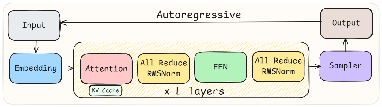
The image is a technical block diagram illustrating the architecture and data flow of an autoregressive model, likely a transformer-based language model. It shows the sequential processing steps from input to output, with a feedback loop characteristic of autoregressive generation. The diagram uses color-coded blocks and directional arrows to represent components and data flow.
### Components/Axes
The diagram is structured as a flowchart with the following labeled components, listed in order of data flow:
1. **Input** (Light gray block, top-left)
2. **Embedding** (Light blue block, below Input)
3. **Central Processing Block** (Large, beige block with diagonal hatching, center):
* **Attention** (Pink block, left side of central block)
* Contains a sub-label: **KV Cache** (Small, light blue block within the Attention block)
* **All Reduce RMSNorm** (Yellow block, to the right of Attention)
* **FFN** (Light green block, to the right of the first RMSNorm)
* **All Reduce RMSNorm** (Yellow block, to the right of FFN)
* Label at the bottom of the central block: **x L layers**
4. **Sampler** (Light purple block, right of the central block)
5. **Output** (Light gray block, top-right)
6. **Process Label**: The text **Autoregressive** is centered at the top of the diagram, above the main flow.
**Spatial Grounding & Flow:**
* The primary data flow is from left to right: `Input` → `Embedding` → `Central Processing Block` → `Sampler` → `Output`.
* A feedback arrow runs from the top of the `Output` block back to the `Input` block, labeled by the overarching **Autoregressive** title. This indicates the model's output is fed back as input for the next generation step.
* The `Central Processing Block` is the core computational unit, indicated to be repeated **x L layers** deep.
### Detailed Analysis
**Component Transcription & Relationships:**
* **Input**: The entry point for the model, receiving data (e.g., a token sequence).
* **Embedding**: Converts discrete input tokens into continuous vector representations.
* **Central Processing Block (x L layers)**: This represents one transformer block, repeated `L` times. The internal flow within this block is sequential:
1. **Attention**: Performs self-attention operations. The embedded **KV Cache** sub-component is noted, which is a standard optimization for autoregressive inference to store Key and Value states from previous steps.
2. **All Reduce RMSNorm**: Applies Root Mean Square Layer Normalization. The "All Reduce" prefix suggests this normalization may be synchronized across multiple devices in a distributed training/inference setup.
3. **FFN**: The Feed-Forward Network, a position-wise fully connected layer.
4. **All Reduce RMSNorm**: A second application of the synchronized RMSNorm, likely following the FFN (a common transformer design pattern).
* **Sampler**: Takes the final hidden states from the last transformer layer and samples or selects the next token (e.g., via argmax or top-k sampling).
* **Output**: The generated token, which is then fed back into the `Input` for the next autoregressive step.
### Key Observations
1. **Explicit Autoregressive Loop**: The diagram explicitly visualizes the core autoregressive property with the feedback arrow from `Output` to `Input`.
2. **Distributed Training Cue**: The repeated use of **"All Reduce"** in the normalization layers is a significant detail. It strongly implies the architecture is designed for or depicted in the context of model parallelism or distributed training, where gradient or activation statistics are synchronized across multiple processors.
3. **Layer Repetition**: The **"x L layers"** label clearly indicates the depth of the model's core processing stack.
4. **KV Cache Integration**: The inclusion of the **KV Cache** within the Attention block highlights a critical optimization for efficient autoregressive inference, preventing recomputation of past key and value vectors.
### Interpretation
This diagram provides a high-level, functional schematic of a modern autoregressive transformer model, with specific annotations pointing to practical implementation details.
* **What it demonstrates**: It shows the standard pipeline: input embedding, repeated transformer layers (each with attention and FFN sub-layers, interspersed with normalization), and a final sampling step. The feedback loop encapsulates the sequential, token-by-token generation process.
* **How elements relate**: The flow is strictly sequential and cyclic. The `Central Processing Block` is the computational engine, its internal components (Attention → Norm → FFN → Norm) represent the standard pre-norm transformer block design. The `Sampler` acts as the decision-making head.
* **Notable Anomalies/Details**: The most notable technical detail is the **"All Reduce"** prefix on the RMSNorm layers. This is not part of the standard transformer architecture description but is a crucial implementation detail for large-scale distributed systems. It suggests the diagram is not just a theoretical model but is concerned with the practicalities of training or running very large models across multiple hardware units. The explicit mention of the **KV Cache** further grounds the diagram in the context of efficient inference systems.
In summary, this is a technically precise diagram of an autoregressive transformer, emphasizing its layered structure, cyclic generation process, and specific design choices (`All Reduce` norms, `KV Cache`) relevant to high-performance, distributed computing environments.