## Chart: Density Plot by Sex
### Overview
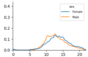
The image is a density plot comparing the distribution of a variable (unspecified) between females and males. The plot shows the probability density of the variable along the x-axis, with separate lines for each sex.
### Components/Axes
* **X-axis:** Ranges from 0 to 22, with tick marks at intervals of 5. The variable represented by the x-axis is not explicitly labeled.
* **Y-axis:** Ranges from 0.0 to 0.4, with tick marks at intervals of 0.1. Represents the density.
* **Legend:** Located in the top-right corner.
* **Female:** Represented by a blue line.
* **Male:** Represented by an orange line.
### Detailed Analysis
* **Female (Blue Line):**
* The density starts near 0 at x=0.
* The density increases, peaking around x=12 with a density of approximately 0.13.
* The density then decreases, approaching 0 around x=22.
* **Male (Orange Line):**
* The density starts near 0 at x=0.
* The density increases, peaking around x=11 with a density of approximately 0.14.
* The density then decreases, approaching 0 around x=22.
### Key Observations
* Both distributions are unimodal (single peak).
* The male distribution peaks slightly earlier (around x=11) than the female distribution (around x=12).
* The peak density for males is slightly higher (0.14) than for females (0.13).
* Both distributions have similar shapes and ranges.
### Interpretation
The density plot suggests that the variable being analyzed has a similar distribution for both males and females. However, there is a slight tendency for males to have lower values of the variable compared to females, as indicated by the earlier peak in the male distribution. The variable itself is not specified in the image, so further context is needed to understand the significance of this difference.