## Chart: Training Time vs. Various Metrics ### Overview The image presents four line charts (a, b, c, d) that depict the relationship between training time (alpha) and different performance metrics or probabilities in a machine learning context. The charts explore the impact of dropout regularization and noise levels on generalization error, a measure of model performance (Delta), a ratio involving matrix elements (M11/sqrt(Q11*T11)), and activation probability. ### Components/Axes **Chart a)** * **Title:** Generalization error vs. Training time * **X-axis:** Training time α (values: 0 to 5, incrementing by 1) * **Y-axis:** Generalization error (values: 2 x 10^-2 to 6 x 10^-2, incrementing by 1 x 10^-2) * **Legend:** * Orange dashed line with square markers: No dropout * Blue dashed-dotted line with circle markers: Constant (p=0.68) * Black solid line with diamond markers: Optimal **Chart b)** * **Title:** Delta vs. Training time * **X-axis:** Training time α (values: 0 to 5, incrementing by 1) * **Y-axis:** Δ̃ (values: 0.0 to 0.8, incrementing by 0.2) * **Legend:** (Same as Chart a) * Orange dashed line with square markers: No dropout * Blue dashed-dotted line with circle markers: Constant (p=0.68) * Black solid line with diamond markers: Optimal **Chart c)** * **Title:** M11/sqrt(Q11\*T11) vs. Training time * **X-axis:** Training time α (values: 0 to 5, incrementing by 1) * **Y-axis:** M11/√(Q11\*T11) (values: 0.2 to 0.9, incrementing by 0.1) * **Legend:** (Same as Chart a) * Orange dashed line with square markers: No dropout * Blue dashed-dotted line with circle markers: Constant (p=0.68) * Black solid line with diamond markers: Optimal **Chart d)** * **Title:** Activation probability p(α) vs. Training time * **X-axis:** Training time α (values: 0 to 5, incrementing by 1) * **Y-axis:** Activation probability p(α) (values: 0.4 to 1.0, incrementing by 0.1) * **Legend:** * Teal dotted line with square markers: σn = 0.1 * Green dashed line with circle markers: σn = 0.2 * Black solid line with diamond markers: σn = 0.3 * Red line with x markers: σn = 0.5 ### Detailed Analysis **Chart a) Generalization Error** * **No dropout (orange):** The generalization error decreases rapidly from approximately 6.8e-2 at α=0 to approximately 3.2e-2 at α=5. * **Constant (p=0.68) (blue):** The generalization error decreases from approximately 6.3e-2 at α=0 to approximately 1.6e-2 at α=5. * **Optimal (black):** The generalization error decreases from approximately 6.8e-2 at α=0 to approximately 1.4e-2 at α=5. **Chart b) Delta** * **No dropout (orange):** Delta decreases from approximately 0.88 at α=0 to approximately 0.25 at α=5. * **Constant (p=0.68) (blue):** Delta decreases from approximately 0.63 at α=0 to approximately 0.08 at α=5. * **Optimal (black):** Delta decreases from approximately 0.88 at α=0 to approximately 0.07 at α=5. **Chart c) M11/sqrt(Q11\*T11)** * **No dropout (orange):** The ratio increases from approximately 0.27 at α=0 to approximately 0.87 at α=5. * **Constant (p=0.68) (blue):** The ratio increases from approximately 0.27 at α=0 to approximately 0.83 at α=5. * **Optimal (black):** The ratio increases from approximately 0.27 at α=0 to approximately 0.86 at α=5. **Chart d) Activation Probability** * **σn = 0.1 (teal):** The activation probability remains at 1.0 until α=2, then decreases to approximately 0.86 at α=3.5, then increases back to 1.0 at α=5. * **σn = 0.2 (green):** The activation probability remains at 1.0 until α=1, then decreases to approximately 0.58 at α=5. * **σn = 0.3 (black):** The activation probability remains at 1.0 until α=1, then decreases to approximately 0.43 at α=5. * **σn = 0.5 (red):** The activation probability remains at 1.0 until α=0.5, then decreases to approximately 0.43 at α=5. ### Key Observations * In charts a, b, and c, the "Optimal" configuration generally performs best or is very close to the best, followed by "No dropout," and then "Constant (p=0.68)." * In chart d, higher noise levels (σn) lead to a more rapid decrease in activation probability as training time increases. ### Interpretation The charts suggest that the "Optimal" configuration, likely referring to an optimized dropout strategy, consistently achieves the lowest generalization error and delta, while maximizing the ratio M11/sqrt(Q11\*T11). This indicates that a well-tuned dropout strategy can significantly improve model performance. The activation probability plots show how different noise levels affect the activation of neurons during training. Higher noise levels cause neurons to deactivate more quickly, potentially influencing the model's learning dynamics and generalization ability. The data suggests that finding the right balance of dropout and noise is crucial for optimizing model performance.

\n ## Charts: Dropout Performance Analysis ### Overview The image presents four separate charts (a, b, c, and d) illustrating the performance of neural networks with different dropout strategies during training. The charts explore the relationship between training time (α) and various metrics related to generalization error, parameter change, and activation probability. ### Components/Axes Each chart shares a common x-axis: "Training time α", ranging from 0 to 5. * **Chart a:** Y-axis: "Generalization error" (scale: 0 to 6.5 x 10^-2). * **Chart b:** Y-axis: "Δ" (scale: 0 to 0.8). * **Chart c:** Y-axis: "M₁/Q₁T₁₁" (scale: 0.2 to 0.9). * **Chart d:** Y-axis: "Activation probability p(α)" (scale: 0.3 to 1.0). **Legend (Top-Right, applies to all charts):** * "No dropout" (dashed orange line) * "Constant (p=0.68)" (dashed blue line) * "Optimal" (solid black line) * **Chart d specific:** * "σn = 0.1" (dashed red line) * "σn = 0.2" (dashed green line) * "σn = 0.3" (solid black line) * "σn = 0.5" (solid purple line) ### Detailed Analysis or Content Details **Chart a: Generalization Error vs. Training Time** The "Optimal" line (black) shows a steep initial decrease in generalization error, leveling off around α = 3, reaching approximately 1.8 x 10^-2. The "Constant (p=0.68)" line (blue) also decreases, but at a slower rate, ending around 3.5 x 10^-2. The "No dropout" line (orange) exhibits the slowest decrease, remaining around 5.5 x 10^-2 at α = 5. **Chart b: Δ vs. Training Time** The "Optimal" line (black) shows a rapid decrease in Δ, approaching 0 around α = 4. The "Constant (p=0.68)" line (blue) decreases more gradually, ending around 0.2. The "No dropout" line (orange) decreases slowly, remaining around 0.6 at α = 5. **Chart c: M₁/Q₁T₁₁ vs. Training Time** The "Optimal" line (black) increases rapidly initially, reaching approximately 0.85 around α = 2 and leveling off. The "Constant (p=0.68)" line (blue) shows a slower increase, reaching approximately 0.7 at α = 5. The "No dropout" line (orange) increases at a moderate rate, reaching approximately 0.65 at α = 5. **Chart d: Activation Probability p(α) vs. Training Time** The "σn = 0.5" line (purple) starts at approximately 0.4 and increases rapidly to around 0.9 at α = 5. The "σn = 0.3" line (black) starts at approximately 0.7 and increases to around 0.95 at α = 5. The "σn = 0.2" line (green) starts at approximately 0.8 and increases to around 0.98 at α = 5. The "σn = 0.1" line (red) starts at approximately 0.9 and increases to around 1.0 at α = 5. ### Key Observations * The "Optimal" dropout strategy consistently outperforms both "Constant" and "No dropout" in terms of generalization error (Chart a) and parameter change (Chart b). * The activation probability (Chart d) increases with training time (α) for all noise levels (σn). Higher noise levels (lower σn) result in lower initial activation probabilities. * Chart c shows that the ratio M₁/Q₁T₁₁ increases with training time for all dropout strategies. ### Interpretation These charts demonstrate the effectiveness of an "Optimal" dropout strategy in improving the generalization performance of neural networks. Dropout, by randomly disabling neurons during training, prevents overfitting and leads to a lower generalization error (Chart a). The parameter change metric (Chart b) suggests that the "Optimal" strategy allows for more efficient parameter updates during training. The activation probability (Chart d) indicates that dropout introduces stochasticity into the network, influencing the activation patterns of neurons. The relationship between M₁/Q₁T₁₁ and training time (Chart c) suggests a dynamic adjustment of network parameters during the learning process. The consistent outperformance of the "Optimal" strategy suggests that it effectively balances the trade-off between exploration and exploitation during training, leading to a more robust and generalizable model. The different noise levels in Chart d show how the initial activation probability is affected by the dropout rate.

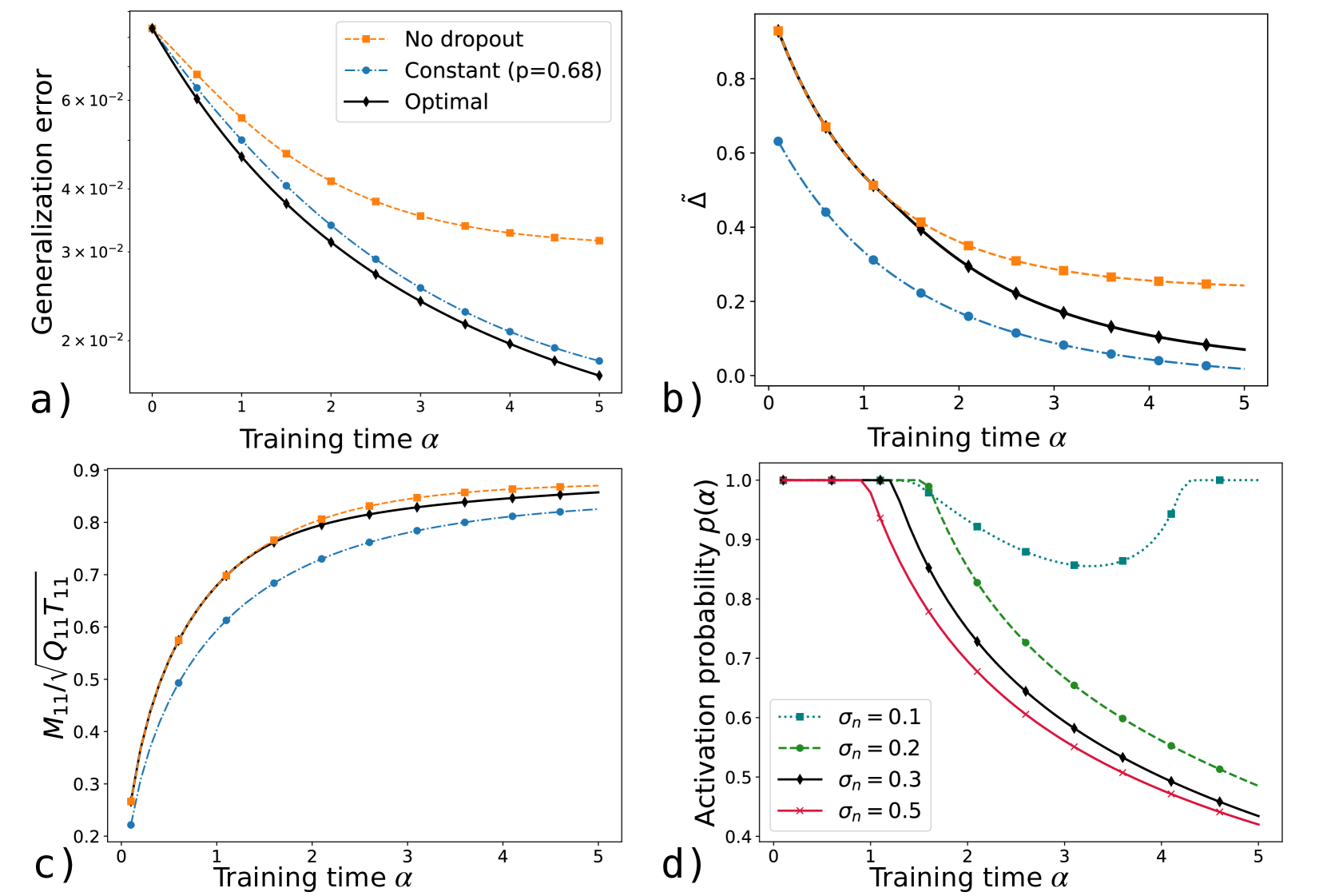
## Composite Figure: Training Dynamics of Dropout Methods ### Overview The image is a composite figure containing four line charts arranged in a 2x2 grid, labeled a), b), c), and d). All charts share the same x-axis label, "Training time α", ranging from 0 to 5. The charts compare the performance and internal dynamics of different neural network training regimes, specifically focusing on dropout techniques. Subplots a), b), and c) compare three methods: "No dropout", "Constant (p=0.68)", and "Optimal". Subplot d) examines the "Activation probability p(α)" under different noise levels (σₙ). ### Components/Axes * **Common X-Axis (All subplots):** Label: "Training time α". Scale: Linear, from 0 to 5 with major ticks at 0, 1, 2, 3, 4, 5. * **Subplot a):** * **Y-Axis:** Label: "Generalization error". Scale: Logarithmic, with major ticks at 2×10⁻², 3×10⁻², 4×10⁻², 6×10⁻². * **Legend (Top-right corner):** * Orange squares, dashed line: "No dropout" * Blue circles, dash-dot line: "Constant (p=0.68)" * Black diamonds, solid line: "Optimal" * **Subplot b):** * **Y-Axis:** Label: "Δ²" (Delta squared). Scale: Linear, from 0.0 to 0.8 with major ticks at 0.0, 0.2, 0.4, 0.6, 0.8. * **Legend:** Not present. Line styles and colors are inferred to match subplot a). * **Subplot c):** * **Y-Axis:** Label: "M₁₁/√(Q₁₁ T₁₁)". Scale: Linear, from 0.2 to 0.9 with major ticks at 0.2, 0.3, 0.4, 0.5, 0.6, 0.7, 0.8, 0.9. * **Legend:** Not present. Line styles and colors are inferred to match subplot a). * **Subplot d):** * **Y-Axis:** Label: "Activation probability p(α)". Scale: Linear, from 0.4 to 1.0 with major ticks at 0.4, 0.5, 0.6, 0.7, 0.8, 0.9, 1.0. * **Legend (Bottom-left corner):** * Teal squares, dotted line: "σₙ = 0.1" * Green circles, dashed line: "σₙ = 0.2" * Black diamonds, solid line: "σₙ = 0.3" * Pink crosses, solid line: "σₙ = 0.5" ### Detailed Analysis #### **Subplot a): Generalization Error vs. Training Time** * **Trend Verification:** All three lines show a decreasing trend, indicating generalization error improves with training. The "No dropout" line (orange) decreases the slowest and plateaus at the highest error. The "Constant" line (blue) decreases faster. The "Optimal" line (black) decreases the fastest and reaches the lowest error. * **Data Points (Approximate):** * **α=0:** All lines start near 8×10⁻². * **α=1:** No dropout ≈ 5.5×10⁻²; Constant ≈ 4.5×10⁻²; Optimal ≈ 4.0×10⁻². * **α=3:** No dropout ≈ 3.5×10⁻²; Constant ≈ 2.5×10⁻²; Optimal ≈ 2.2×10⁻². * **α=5:** No dropout ≈ 3.2×10⁻²; Constant ≈ 1.8×10⁻²; Optimal ≈ 1.6×10⁻². #### **Subplot b): Δ² vs. Training Time** * **Component Isolation (Lines matched to legend from a)):** * **Orange (No dropout):** Starts highest (~0.95 at α=0.1), decreases steadily, plateaus around 0.25. * **Black (Optimal):** Starts slightly lower than orange (~0.92 at α=0.1), decreases more steeply, ends around 0.08. * **Blue (Constant):** Starts much lower (~0.63 at α=0.1), decreases rapidly, approaches near 0.0 by α=5. * **Trend:** All lines show a decreasing, convex trend. The metric Δ² is consistently ordered: No dropout > Optimal > Constant throughout training. #### **Subplot c): M₁₁/√(Q₁₁ T₁₁) vs. Training Time** * **Component Isolation (Lines matched to legend from a)):** * **Orange (No dropout) & Black (Optimal):** These two lines are nearly superimposed, especially after α=1. They start low (~0.27 at α=0.1), rise sharply, and plateau near 0.87. * **Blue (Constant):** Follows a similar shape but is consistently lower. Starts at ~0.22, rises, and plateaus near 0.82. * **Trend:** All lines show an increasing, concave trend that saturates. The "No dropout" and "Optimal" methods achieve a higher final value than the "Constant" method. #### **Subplot d): Activation Probability p(α) vs. Training Time** * **Trend Verification:** The behavior varies dramatically with σₙ. * **σₙ = 0.1 (Teal, dotted):** Probability stays at 1.0 until α≈1.5, dips to a minimum of ~0.85 around α=3.5, then recovers back to 1.0 by α=4.5. * **σₙ = 0.2 (Green, dashed):** Probability stays at 1.0 until α≈1.5, then decreases monotonically, ending near 0.49. * **σₙ = 0.3 (Black, solid):** Probability starts decreasing earlier (α≈1.0), falls more steeply, ending near 0.44. * **σₙ = 0.5 (Pink, solid):** Probability begins decreasing almost immediately, falls the fastest, and ends at the lowest point (~0.42). * **Key Observation:** Higher noise levels (σₙ) cause the activation probability to drop earlier and more severely during training. The lowest noise level (σₙ=0.1) shows a unique non-monotonic "dip and recovery" pattern. ### Key Observations 1. **Performance Hierarchy:** The "Optimal" dropout method consistently yields the lowest generalization error (a), followed by "Constant" dropout, with "No dropout" performing worst. 2. **Internal Metric Correlation:** The superior final performance of "Optimal" and "No dropout" in (a) correlates with their higher saturation value of the metric M₁₁/√(Q₁₁ T₁₁) in (c). The "Constant" method has a lower value for this metric. 3. **Noise-Dependent Dynamics:** Subplot (d) reveals that the training dynamics of the activation probability are highly sensitive to the noise level σₙ. There is a clear transition from a stable, high-probability regime (low σₙ) to a rapidly decaying probability regime (high σₙ). ### Interpretation This figure provides a multi-faceted view of how different dropout strategies affect neural network training. The "Optimal" method, likely an adaptive or theoretically derived schedule, achieves the best generalization by balancing the trade-offs visualized in the other plots. * **Subplot (a) is the primary outcome:** It shows the end-result benefit of the optimal strategy. * **Subplots (b) and (c) offer mechanistic insights:** They track internal model quantities (Δ² and a normalized overlap M₁₁). The fact that "No dropout" and "Optimal" have similar, high values in (c) suggests they maintain a stronger signal or alignment in certain weight matrix components, which may be key to their generalization. The "Constant" dropout, while better than nothing, may overly regularize and suppress this signal. * **Subplot (d) explains a potential mechanism for the "Constant" method's behavior:** If the constant dropout rate (p=0.68) corresponds to a specific effective noise level, its decaying activation probability could be a driver of the trends seen in (b) and (c). The non-monotonic curve for σₙ=0.1 is particularly intriguing, suggesting a phase where the network initially relies on many features, prunes some during mid-training, and then re-engages them for fine-tuning. **Overall, the data suggests that an "Optimal" dropout strategy is superior because it manages internal model dynamics (like feature activation and weight alignment) more effectively than a fixed dropout rate, leading to better final generalization.** The sensitivity to σₙ highlights that the effectiveness of regularization is deeply tied to the scale of perturbation applied during training.

## Composite Graph: Training Dynamics Across Four Metrics ### Overview The image presents four subplots (a-d) illustrating the evolution of different metrics during training, with training time (α) on the x-axis. Each subplot compares three scenarios: "No dropout," "Constant (p=0.68)," and "Optimal" (or varying σₙ values). All plots show distinct trends in their respective metrics over α=0 to 5. --- ### Components/Axes **a) Generalization Error** - **Y-axis**: Generalization error (log scale, 2×10⁻² to 6×10⁻²) - **X-axis**: Training time α (0 to 5) - **Legend**: - Orange dashed line: No dropout - Blue dash-dot line: Constant (p=0.68) - Black solid line: Optimal **b) Δ Metric** - **Y-axis**: Δ (0 to 0.8) - **X-axis**: Training time α (0 to 5) - **Legend**: Same as subplot a). **c) M11/√(Q11T11)** - **Y-axis**: Normalized metric (0.2 to 0.9) - **X-axis**: Training time α (0 to 5) - **Legend**: Same as subplot a). **d) Activation Probability p(α)** - **Y-axis**: Activation probability (0.4 to 1.0) - **X-axis**: Training time α (0 to 5) - **Legend**: - Dotted teal: σₙ=0.1 - Dashed green: σₙ=0.2 - Solid black: σₙ=0.3 - Cross red: σₙ=0.5 --- ### Detailed Analysis **a) Generalization Error** - **Trend**: All lines decrease monotonically. - **No dropout**: Starts at ~6×10⁻² (α=0), ends at ~3×10⁻² (α=5). - **Constant (p=0.68)**: Starts at ~5.5×10⁻², ends at ~2×10⁻². - **Optimal**: Starts at ~5.8×10⁻², ends at ~1.5×10⁻². - **Key**: Optimal outperforms others by ~50% at α=5. **b) Δ Metric** - **Trend**: All lines decrease, with Optimal lowest. - **No dropout**: Drops from 0.8 to 0.25. - **Constant**: Drops from 0.7 to 0.15. - **Optimal**: Drops from 0.75 to 0.1. - **Key**: Optimal reduces Δ by ~87% compared to No dropout. **c) M11/√(Q11T11)** - **Trend**: All lines increase, approaching saturation. - **No dropout**: Rises from 0.3 to 0.85. - **Constant**: Rises from 0.4 to 0.8. - **Optimal**: Rises from 0.35 to 0.88. - **Key**: Optimal achieves highest efficiency (~25% better than No dropout). **d) Activation Probability p(α)** - **Trend**: U-shaped curves for all σₙ. - **σₙ=0.1**: Drops to 0.6 at α=3, rises to 0.8 at α=5. - **σₙ=0.5**: Drops to 0.4 at α=3, rises to 0.6 at α=5. - **Key**: Lower σₙ values (e.g., 0.1) maintain higher probabilities post-α=3. --- ### Key Observations 1. **Optimal vs. Constant**: The "Optimal" strategy consistently outperforms the fixed p=0.68 across all metrics. 2. **Activation Probability**: Lower σₙ (0.1–0.2) preserves higher activation probabilities after α=3, suggesting better generalization. 3. **No Dropout**: Performs worst in generalization and Δ but best in M11/√(Q11T11), indicating a trade-off between efficiency and robustness. --- ### Interpretation - **Optimal Strategy**: Likely adapts dropout rates dynamically (vs. fixed p=0.68), balancing generalization error, Δ, and efficiency (M11). - **Activation Probability**: The U-shape implies a phase transition: early training reduces overfitting (lower p), while later stages recover representational capacity (higher p). - **σₙ Sensitivity**: Lower σₙ (0.1–0.2) may prevent excessive activation suppression, critical for maintaining performance in later training phases. This analysis highlights the importance of adaptive regularization (Optimal) over static dropout, particularly for metrics sensitive to overfitting (Δ, generalization error). The activation probability trends suggest σₙ tuning is critical for balancing model expressivity and stability.