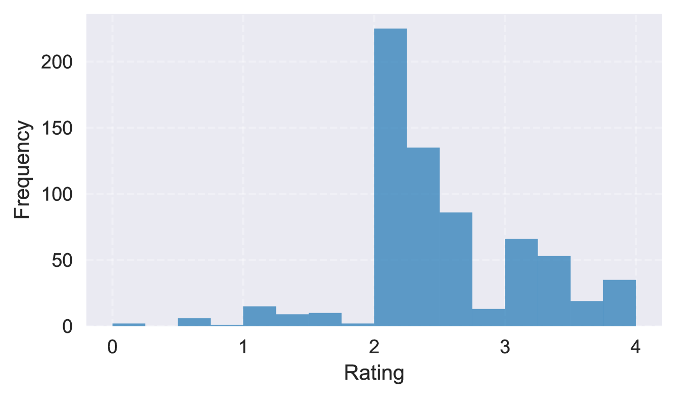
## Histogram: Rating Frequency Distribution ### Overview The image displays a histogram visualizing the distribution of ratings across a scale from 0 to 4. The y-axis represents frequency, with the highest bar centered at a rating of 2.0, indicating a concentration of data points around this value. Frequencies decrease significantly at the extremes (0 and 4). ### Components/Axes - **X-axis (Rating)**: Labeled "Rating," with discrete intervals marked at 0, 1, 2, 3, and 4. The scale is linear, with equal spacing between intervals. - **Y-axis (Frequency)**: Labeled "Frequency," ranging from 0 to 200 in increments of 50. The axis is continuous. - **Bars**: Blue-colored bars represent frequency counts for each rating interval. No legend is present, as the chart uses a single color for all data. ### Detailed Analysis - **Rating 0**: Minimal frequency (~2–5), with a single bar barely visible above the baseline. - **Rating 1**: Slightly higher frequency (~10–15), with a short bar. - **Rating 2**: Dominant peak with a frequency of approximately **220**, the tallest bar in the chart. - **Rating 3**: Moderate frequency (~60–70), with a bar shorter than the peak at 2.0. - **Rating 4**: Low frequency (~30–40), with a bar shorter than the peak at 3.0. ### Key Observations 1. **Central Peak**: The distribution is heavily skewed toward a rating of 2.0, which accounts for the majority of data points. 2. **Bimodal Tendency**: While not strictly bimodal, there are secondary peaks at ratings 3.0 and 4.0, though significantly lower than the central peak. 3. **Extreme Rarity**: Ratings 0 and 1 are underrepresented, suggesting these values are outliers or less common in the dataset. ### Interpretation The data suggests a strong central tendency around a rating of 2.0, possibly indicating a consensus or common perception among respondents. The lower frequencies at the extremes (0 and 1) may reflect dissatisfaction or disengagement, while the moderate frequencies at 3.0 and 4.0 could represent positive but less dominant opinions. The absence of a legend simplifies interpretation but limits contextual understanding of the data source (e.g., survey, product reviews). The distribution’s shape might imply a need for further analysis to identify factors influencing the central peak or outliers.