\n
## Diagram: Deep-Thinking Regime - Layer-wise Distribution Comparison
### Overview
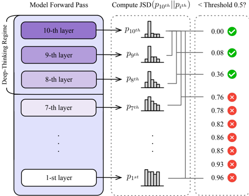
The image is a technical diagram illustrating a process called the "Deep-Thinking Regime" within a neural network model. It visualizes how the probability distribution output from the final (10th) layer is compared to the distributions from all preceding layers using the Jensen-Shannon Divergence (JSD). The diagram shows which layers produce distributions sufficiently similar to the final output (below a threshold) and which do not.
### Components/Axes
The diagram is organized into three vertical sections from left to right:
1. **Left Section - Model Forward Pass:**
* A large, light purple rounded rectangle labeled **"Deep-Thinking Regime"** on its left side.
* Inside, a vertical stack of rounded rectangles representing model layers, from top to bottom:
* `10-th layer` (dark purple)
* `9-th layer` (medium purple)
* `8-th layer` (light purple)
* `7-th layer` (very light purple)
* `...` (ellipsis indicating omitted layers)
* `1-st layer` (white)
* Each layer box has an arrow pointing to the right, towards a corresponding probability distribution.
2. **Middle Section - Probability Distributions:**
* A column of small histogram-like icons, each labeled with a probability distribution notation:
* `p_10th` (top)
* `p_9th`
* `p_8th`
* `p_7th`
* `...`
* `p_1st` (bottom)
* These icons represent the output probability distributions from each respective layer.
3. **Right Section - JSD Computation & Threshold Check:**
* A header at the top reads: **"Compute JSD(p_10th || p_nth) < Threshold 0.5?"**
* A vertical list of numerical values, each connected by a line to the comparison between `p_10th` and a lower layer's distribution (`p_nth`):
* `0.00` (connected to `p_9th`)
* `0.08` (connected to `p_8th`)
* `0.36` (connected to `p_7th`)
* `0.76`
* `0.78`
* `0.82`
* `0.86`
* `0.85`
* `0.93`
* `0.96` (connected to `p_1st`)
* To the right of each number is a status symbol:
* A green circle with a white checkmark (✅) for values `0.00`, `0.08`, and `0.36`.
* A red circle with a white 'X' (❌) for all values from `0.76` to `0.96`.
### Detailed Analysis
* **Process Flow:** The diagram depicts a forward pass through a 10-layer model operating in a "Deep-Thinking Regime." For each layer `n` (from 9 down to 1), the Jensen-Shannon Divergence (JSD) is calculated between the final layer's distribution (`p_10th`) and that layer's distribution (`p_nth`).
* **Threshold Comparison:** The computed JSD value is compared against a fixed threshold of `0.5`.
* **Results:**
* **Layers 9, 8, and 7:** The JSD values (`0.00`, `0.08`, `0.36`) are all **less than 0.5**, resulting in a green checkmark. This indicates their output distributions are considered "similar" to the final layer's distribution.
* **Layers 6 through 1:** The JSD values (`0.76` to `0.96`) are all **greater than 0.5**, resulting in a red 'X'. This indicates their output distributions are significantly different from the final layer's distribution.
* **Trend Verification:** There is a clear visual and numerical trend. As we move from the top (layer 9) to the bottom (layer 1), the JSD value **consistently increases** (with a minor fluctuation from 0.86 to 0.85). This corresponds to the visual transition from green checkmarks to red crosses, showing that lower layers diverge more from the final output.
### Key Observations
1. **Sharp Transition:** There is a distinct cutoff after the 7th layer. The 7th layer is the last one with a JSD below the threshold (`0.36`), while the next measured layer (implied 6th) jumps to `0.76`.
2. **Monotonic Increase (Approximate):** The JSD generally increases with layer depth (lower layer number), suggesting that representations become progressively less like the final output as we go earlier in the network.
3. **Perfect Similarity:** The JSD between `p_10th` and `p_9th` is `0.00`, indicating these two distributions are considered identical by this metric.
4. **Spatial Layout:** The legend (checkmarks/crosses) is positioned on the far right, directly adjacent to the numerical results they qualify. The "Deep-Thinking Regime" label is vertically centered on the left edge of the layer stack.
### Interpretation
This diagram illustrates a diagnostic or analytical technique for understanding the internal processing of a neural network. The "Deep-Thinking Regime" likely refers to a specific mode of operation or a model architecture designed for interpretability.
* **What it suggests:** The data demonstrates that in this regime, the model's "thinking" or representational state stabilizes in the upper layers (7-10). The final output distribution (`p_10th`) is already largely formed by the 7th layer, as evidenced by the low JSD. The lower layers (1-6) are processing information in a way that is fundamentally different from the final decision layer.
* **How elements relate:** The layers are the source of data (distributions), the JSD is the comparison metric, and the threshold is the decision rule. The flow is strictly top-down for comparison (always against the final layer).
* **Notable implications:** This could be used to identify a "sufficient depth" for feature extraction, to detect layer-wise specialization, or to validate that a "deep-thinking" process is occurring as intended (i.e., later layers refining rather than radically changing the representation). The sharp transition might indicate a phase change in processing between the 7th and 6th layers. The threshold of 0.5 is an arbitrary but critical parameter defining "similarity."