## Diagram: Python Function to Symbolic Representation Transformation
### Overview
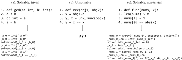
The image is a technical diagram illustrating the transformation of three different Python function definitions into their corresponding symbolic representations, likely for use in a solver or verification system. The diagram is divided into three vertical columns, each labeled with a classification of the function's solvability: (a) Solvable, trivial; (b) Unsolvable; (c) Solvable, non-trivial. Each column contains a Python function at the top, a downward-pointing arrow, and the resulting symbolic code at the bottom.
### Components/Axes
The diagram has three main components arranged horizontally:
1. **Column (a):** Labeled "(a): Solvable, trivial".
2. **Column (b):** Labeled "(b): Unsolvable".
3. **Column (c):** Labeled "(c): Solvable, non-trivial".
Each column contains:
* A Python function definition (lines numbered 1-4).
* A gray downward-pointing arrow indicating transformation.
* A block of symbolic code representing the function's logic.
### Detailed Analysis
#### Column (a): Solvable, trivial
* **Python Function:**
```python
1. def gcd(a: int, b: int):
2. a < b
3. c: int = a
4. a = b
```
* **Symbolic Representation:**
```python
_a_0 = Int('_a_0')
_b_0 = Int('_b_0')
solver.add(_a_0 < _b_0)
_c_0 = Int('_c_0')
solver.add(_c_0 == _a_0)
_a_1 = Int('_a_1')
solver.add(_a_1 == _b_0)
```
* **Analysis:** This function appears to be a simplified or partial implementation of a greatest common divisor (GCD) algorithm. The symbolic translation is direct: each variable (`a`, `b`, `c`) is declared as an integer (`Int`), and each operation or assignment is added as a constraint to a `solver`. The logic is linear and contains no loops or complex conditions, hence classified as "trivial".
#### Column (b): Unsolvable
* **Python Function:**
```python
1. def xxx(obj1, obj2):
2. x = obj1.a
3. y, z = unk_func(obj2)
4. y + z == x
```
* **Symbolic Representation:**
```
???
```
* **Analysis:** The function `xxx` accesses an attribute `obj1.a` and calls an unknown function `unk_func(obj2)`, which returns two values. The final line is a comparison (`y + z == x`). The symbolic representation is marked with "???", indicating that the transformation cannot be completed. This is likely because `unk_func` is undefined, making the function's behavior non-deterministic or impossible to model symbolically, hence "Unsolvable".
#### Column (c): Solvable, non-trivial
* **Python Function:**
```python
1. def func(nums, x):
2. len(nums) > x
3. nums[1] = 1
4. nums[0] == abs(x)
```
* **Symbolic Representation:**
```python
_nums_0 = Array('_nums_0', IntSort(), IntSort())
_nums_0_len = Int('_nums_0_len')
_x_0 = Int('_x_0')
solver.add(_nums_0_len > _x_0)
_nums_1 = Store(_nums_0, 1, 1)
_nums_1_len = _nums_0_len
solver.add(_nums_1[0] == If(_x_0 > 0, _x_0, -_x_0))
```
* **Analysis:** This function operates on a list `nums` and an integer `x`. It checks a length condition, assigns a value to an index, and compares another index to the absolute value of `x`. The symbolic translation is more complex:
* `nums` is modeled as an `Array` (a symbolic array).
* The length is a separate integer variable `_nums_0_len`.
* The assignment `nums[1] = 1` is modeled using a `Store` operation, creating a new array state `_nums_1`.
* The absolute value `abs(x)` is modeled using an `If` (ternary) condition.
* This involves state changes (array update) and a conditional expression, making it "non-trivial" but still fully modelable, hence "Solvable".
### Key Observations
1. **Classification Logic:** The solvability classification is based on the ability to translate the Python code into a set of declarative constraints for a solver. "Trivial" functions have a 1:1 mapping. "Non-trivial" functions require more complex modeling (e.g., arrays, state). "Unsolvable" functions contain elements that cannot be modeled (e.g., calls to unknown functions).
2. **Symbolic Modeling Patterns:** The diagram demonstrates common patterns for symbolic representation:
* Variables become symbolic constants (`Int`).
* Comparisons and assignments become `solver.add()` constraints.
* Data structures like lists are modeled as `Array` sorts with `Store` operations for updates.
* Built-in functions like `abs()` are expanded into their logical equivalents (`If` condition).
3. **Visual Flow:** The downward arrows in columns (a) and (c) clearly indicate a successful transformation process. The absence of an arrow and the "???" in column (b) visually emphasize the breakdown in the process.
### Interpretation
This diagram serves as a pedagogical or technical reference for program analysis, formal verification, or symbolic execution. It illustrates the boundary between code that can be automatically analyzed by a constraint solver and code that cannot.
* **What it demonstrates:** The core idea is that for automated reasoning about code, the program must be translatable into a formal, declarative model. The diagram shows the translation process for different levels of complexity.
* **Relationship between elements:** The Python code (imperative, operational) is the input. The symbolic code (declarative, constraint-based) is the output. The classification labels describe the feasibility and complexity of this translation.
* **Notable patterns:** The "Unsolvable" case highlights a fundamental limitation: analysis requires knowledge of all components. An unknown function (`unk_func`) acts as a black box, breaking the symbolic model. The "non-trivial" case shows that while more complex, standard programming constructs (arrays, indexing, built-in functions) have established symbolic representations.
* **Underlying purpose:** The image likely aims to explain concepts in automated theorem proving, software verification, or the creation of symbolic execution engines. It answers the question: "What kinds of code can we automatically reason about, and what makes some code harder or impossible to model?"