## Diagram: Two-Dimensional Discrete Grid with Highlighted Region
### Overview
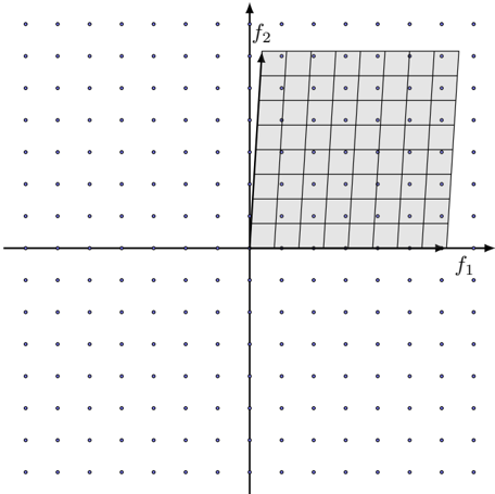
The image is a technical diagram illustrating a two-dimensional coordinate system with a discrete grid of points. A specific rectangular region within the first quadrant is shaded, highlighting a subset of the grid points. The diagram is likely used to conceptualize a domain, search space, or feasible region in fields such as optimization, signal processing, or computational mathematics.
### Components/Axes
* **Coordinate System:** A standard Cartesian plane with two perpendicular axes.
* **Horizontal Axis:** Labeled **\( f_1 \)**. An arrow at the right end indicates the positive direction.
* **Vertical Axis:** Labeled **\( f_2 \)**. An arrow at the top end indicates the positive direction.
* **Origin:** The intersection point of the \( f_1 \) and \( f_2 \) axes.
* **Grid:** A uniform lattice of small, dark blue dots. The dots are spaced at regular intervals along both the horizontal and vertical directions, creating a checkerboard pattern across all four quadrants.
* **Shaded Region:** A light gray, semi-transparent rectangle located in the first quadrant (where both \( f_1 \) and \( f_2 \) are positive).
* **Boundaries:** The region is bounded on the left by the \( f_2 \)-axis and on the bottom by the \( f_1 \)-axis. Its top and right boundaries are straight lines parallel to the axes.
* **Content:** The shaded area overlays and highlights a specific 8x8 sub-grid of the lattice points. The grid points within this region are visually identical to those outside it.
### Detailed Analysis
* **Spatial Grounding:** The shaded region is positioned in the **top-right quadrant** relative to the origin. It starts at the origin (0,0) and extends rightward along the \( f_1 \) axis and upward along the \( f_2 \) axis.
* **Grid Structure:** The grid appears to be an infinite or extensive lattice, as dots continue beyond the visible edges of the image in all directions. The spacing between dots is consistent, suggesting a uniform discretization of the \( f_1 \)-\( f_2 \) plane.
* **Highlighted Subset:** The shaded rectangle precisely encompasses a contiguous block of grid points. Counting the dots along the edges of the shaded area, it contains **8 columns** of dots along the \( f_1 \) direction and **8 rows** of dots along the \( f_2 \) direction, for a total of 64 highlighted points.
* **Textual Content:** The only explicit text in the diagram are the axis labels **\( f_1 \)** and **\( f_2 \)**. No numerical values, scales, legends, or titles are present.
### Key Observations
1. **Conceptual, Not Numerical:** The diagram lacks numerical scales or specific values. It is a schematic representation meant to illustrate a concept rather than present quantitative data.
2. **Discrete vs. Continuous:** It visually contrasts a discrete set of points (the grid) with a continuous area (the shaded rectangle). The shaded area includes all grid points within its continuous boundaries.
3. **First Quadrant Focus:** The highlighting is exclusively in the first quadrant, which often represents positive, feasible, or target values in many technical contexts.
4. **Uniformity:** The perfect regularity of the grid and the rectangular shape of the highlighted region suggest an idealized or simplified model.
### Interpretation
This diagram serves as a visual metaphor for defining a **region of interest within a discrete parameter space**.
* **What it suggests:** The axes \( f_1 \) and \( f_2 \) likely represent two independent variables, features, or parameters. The grid points represent all possible discrete combinations of these parameters. The shaded rectangle defines a specific **subset** or **constraint set**—for example, a feasible region where \( 0 \leq f_1 \leq a \) and \( 0 \leq f_2 \leq b \) for some implicit values \( a \) and \( b \).
* **Relationships:** The diagram establishes a relationship between a global search space (the entire grid) and a local, constrained subspace (the shaded area). It implies that operations, optimizations, or analyses might be restricted to the points within the shaded region.
* **Underlying Concept:** This is a common way to visualize concepts like:
* A **feasible set** in constrained optimization.
* A **support region** for a 2D signal or filter.
* A **search window** in pattern matching or computer vision.
* The **domain** for a function defined on a lattice.
* **Notable Absence:** The lack of specific numbers is intentional. It makes the diagram general and applicable to any situation where a rectangular subset of a 2D grid is relevant. The viewer is meant to understand the *structure* of the relationship, not specific data points.
**In summary, the image is a foundational schematic for understanding how a continuous rectangular constraint defines a discrete subset within a two-dimensional lattice space.**