## Code Comparison Diagram: LLM vs. LLM + APOLLO Theorem Proving
### Overview
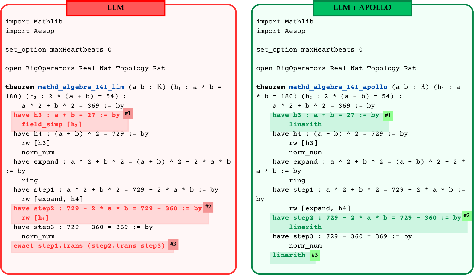
This image is a side-by-side technical diagram comparing two blocks of computer code, specifically written in Lean 4 (a mathematical theorem proving language). The diagram contrasts the output generated by a standard Large Language Model ("LLM") on the left against the output generated by an enhanced system ("LLM + APOLLO") on the right. The image uses color-coding (red for the left panel, green for the right panel) and numbered annotations to highlight specific differences in the proof tactics used to solve the same algebraic theorem.
### Components and Layout
The image is divided into two distinct spatial regions:
1. **Left Panel (Baseline LLM):**
* **Position:** Occupies the left half of the image.
* **Header:** A red rectangular box at the top center containing the text "LLM" in black.
* **Border/Background:** Surrounded by a red border with rounded corners. The background has a very faint pink/red tint.
* **Highlights:** Three specific blocks of code are highlighted with a solid red background and tagged with dark red square labels containing white text: `#1`, `#2`, and `#3`.
2. **Right Panel (Enhanced LLM + APOLLO):**
* **Position:** Occupies the right half of the image.
* **Header:** A green rectangular box at the top center containing the text "LLM + APOLLO" in black.
* **Border/Background:** Surrounded by a dark green border with rounded corners. The background has a very faint green tint.
* **Highlights:** Three specific blocks of code are highlighted with a solid light green background and tagged with dark green square labels containing white text: `#1`, `#2`, and `#3`. These correspond spatially and logically to the highlights in the left panel.
### Content Details
Both panels contain code attempting to prove the same theorem: `mathd_algebra_141`. The setup, imports, and theorem definitions are identical. The differences lie strictly within the highlighted proof tactics.
#### Left Panel Transcription (LLM)
```lean
import Mathlib
import Aesop
set_option maxHeartbeats 0
open BigOperators Real Nat Topology Rat
theorem mathd_algebra_141_llm (a b : ℝ) (h₁ : a * b =
180) (h₂ : 2 * (a + b) = 54) :
a ^ 2 + b ^ 2 = 369 := by
have h3 : a + b = 27 := by #1 [Highlighted Red]
field_simp [h₂] #1 [Highlighted Red]
have h4 : (a + b) ^ 2 = 729 := by
rw [h3]
norm_num
have expand : a ^ 2 + b ^ 2 = (a + b) ^ 2 - 2 * a * b
:= by
ring
have step1 : a ^ 2 + b ^ 2 = 729 - 2 * a * b := by
rw [expand, h4]
have step2 : 729 - 2 * a * b = 729 - 360 := by #2 [Highlighted Red]
rw [h₁] #2 [Highlighted Red]
have step3 : 729 - 360 = 369 := by
norm_num
exact step1.trans (step2.trans step3) #3 [Highlighted Red]
```
#### Right Panel Transcription (LLM + APOLLO)
*Note: Line breaks in the theorem definition differ slightly from the left panel due to text wrapping, but the code logic is identical until the highlights.*
```lean
import Mathlib
import Aesop
set_option maxHeartbeats 0
open BigOperators Real Nat Topology Rat
theorem mathd_algebra_141_apollo (a b : ℝ) (h₁ : a
* b = 180) (h₂ : 2 * (a + b) = 54) :
a ^ 2 + b ^ 2 = 369 := by
have h3 : a + b = 27 := by #1 [Highlighted Green]
linarith #1 [Highlighted Green]
have h4 : (a + b) ^ 2 = 729 := by
rw [h3]
norm_num
have expand : a ^ 2 + b ^ 2 = (a + b) ^ 2 - 2 *
a * b := by
ring
have step1 : a ^ 2 + b ^ 2 = 729 - 2 * a * b :=
by
rw [expand, h4]
have step2 : 729 - 2 * a * b = 729 - 360 := by #2 [Highlighted Green]
linarith #2 [Highlighted Green]
have step3 : 729 - 360 = 369 := by
norm_num
linarith #3 [Highlighted Green]
```
### Key Observations
A direct comparison of the highlighted sections reveals the exact substitutions made by the "APOLLO" system:
* **Highlight #1 Comparison:**
* *LLM (Left):* Uses the tactic `field_simp [h₂]` to prove `a + b = 27`.
* *LLM + APOLLO (Right):* Replaces this with the tactic `linarith`.
* **Highlight #2 Comparison:**
* *LLM (Left):* Uses the tactic `rw [h₁]` (rewrite using hypothesis 1) to prove `729 - 2 * a * b = 729 - 360`.
* *LLM + APOLLO (Right):* Replaces this with the tactic `linarith`.
* **Highlight #3 Comparison:**
* *LLM (Left):* Uses a complex transitive equality chain: `exact step1.trans (step2.trans step3)` to conclude the proof.
* *LLM + APOLLO (Right):* Replaces the entire chain with the single tactic `linarith`.
### Interpretation
This diagram serves as a visual demonstration of the effectiveness of the "APOLLO" system when augmenting a standard LLM for formal theorem proving in Lean 4.
The data suggests that a standard LLM (left panel) attempts to solve mathematical proofs by stringing together highly specific, sometimes overly complex, or potentially incorrect tactics (like `field_simp` for simple linear arithmetic, or manually chaining transitive properties with `exact step1.trans...`). The red highlighting implies these choices are either suboptimal, brittle, or represent hallucinated logic that fails to compile.
Conversely, the "LLM + APOLLO" system (right panel) demonstrates a pattern of simplification and robustness. In all three highlighted instances, APOLLO replaces the LLM's specific tactics with `linarith` (Linear Arithmetic), a powerful and standard automated tactic in Lean designed specifically to solve linear equations and inequalities.
Reading between the lines, APOLLO appears to act as a refinement or correction layer. It recognizes when the base LLM is struggling with basic algebraic manipulations and substitutes a reliable, automated solver (`linarith`), thereby making the proof cleaner, shorter, and mathematically sound. The visual use of red (error/suboptimal) versus green (success/optimal) strongly reinforces the narrative that APOLLO "fixes" the LLM's proof generation.