\n
## Diagram: Comparison of Lean 4 Proof Strategies (LLM vs. LLM + APOLLO)
### Overview
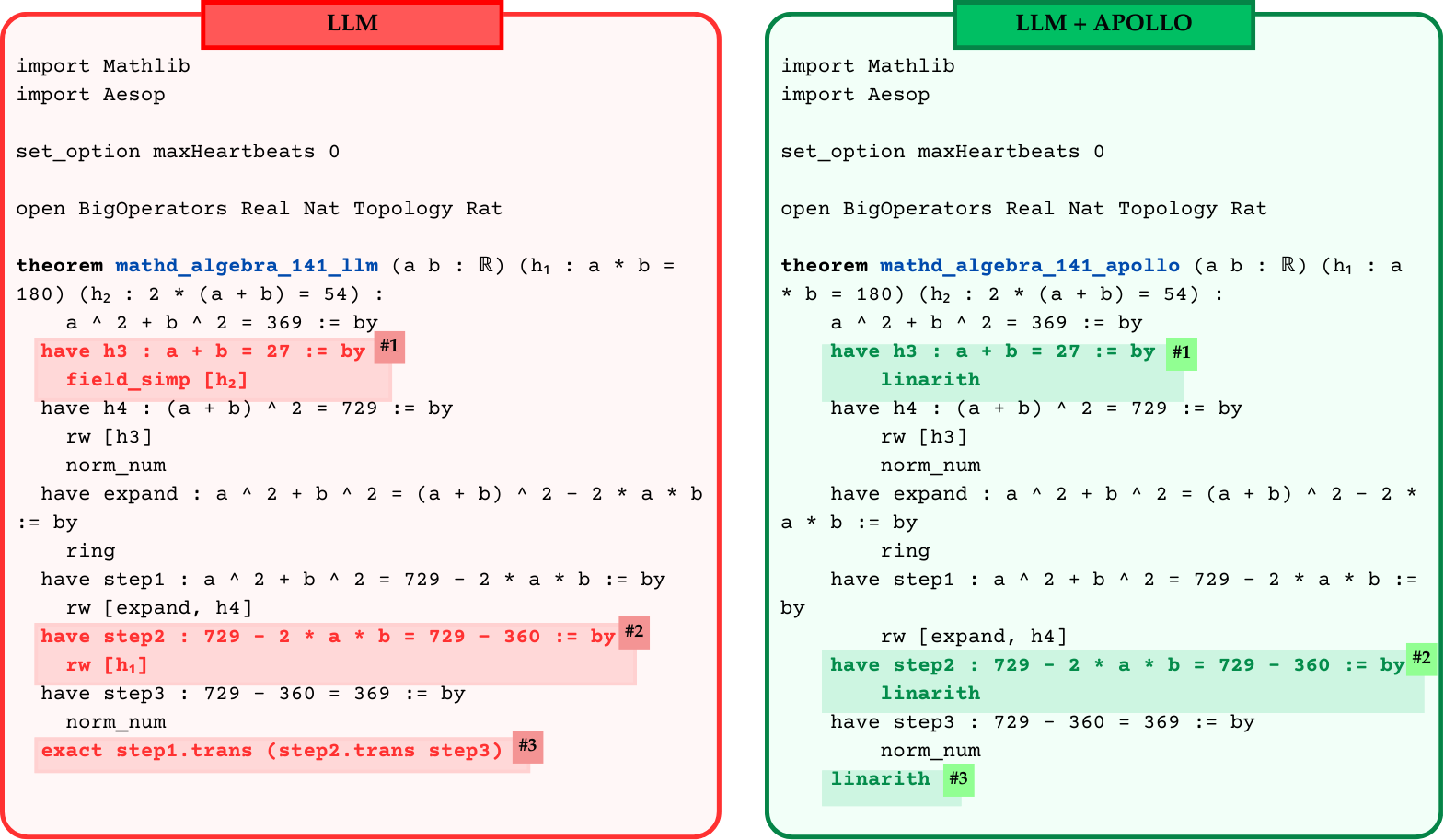
The image presents a side-by-side comparison of two Lean 4 code implementations for proving the same mathematical theorem. The left panel, outlined in red, is labeled "LLM" and shows a proof generated by a Large Language Model. The right panel, outlined in green, is labeled "LLM + APOLLO" and shows a proof that incorporates the APOLLO system. The comparison highlights differences in the tactics and steps used to arrive at the same conclusion.
### Components/Axes
The diagram consists of two primary, vertically oriented rectangular panels:
* **Left Panel (LLM):** Bordered in red. Header text: "LLM".
* **Right Panel (LLM + APOLLO):** Bordered in green. Header text: "LLM + APOLLO".
Each panel contains a block of Lean 4 code. Within the code, specific lines or sequences are highlighted with a background color matching the panel's border (red or green) and are annotated with a numbered tag (e.g., `#1`, `#2`, `#3`).
### Detailed Analysis
Both code blocks begin with identical setup lines and state the same theorem.
**Common Setup & Theorem Statement:**
```lean
import Mathlib
import Aesop
set_option maxHeartbeats 0
open BigOperators Real Nat Topology Rat
theorem mathd_algebra_141_<variant> (a b : ℝ) (h₁ : a * b = 180) (h₂ : 2 * (a + b) = 54) :
a ^ 2 + b ^ 2 = 369 := by
```
* The theorem name differs: `mathd_algebra_141_llm` (left) vs. `mathd_algebra_141_apollo` (right).
* The goal is to prove `a ^ 2 + b ^ 2 = 369` given `a * b = 180` and `2 * (a + b) = 54`.
**Proof Step Comparison:**
| Step / Goal | LLM Proof (Left Panel) | LLM + APOLLO Proof (Right Panel) |
| :--- | :--- | :--- |
| **1. Deduce `a + b = 27`** | `have h3 : a + b = 27 := by` <br> `field_simp [h₂]` <br> *(Highlighted Red, Tag #1)* | `have h3 : a + b = 27 := by` <br> `linarith` <br> *(Highlighted Green, Tag #1)* |
| **2. Compute `(a + b)^2 = 729`** | `have h4 : (a + b) ^ 2 = 729 := by` <br> `rw [h3]` <br> `norm_num` | `have h4 : (a + b) ^ 2 = 729 := by` <br> `rw [h3]` <br> `norm_num` |
| **3. State algebraic identity** | `have expand : a ^ 2 + b ^ 2 = (a + b) ^ 2 - 2 * a * b := by` <br> `ring` | `have expand : a ^ 2 + b ^ 2 = (a + b) ^ 2 - 2 * a * b := by` <br> `ring` |
| **4. Substitute into identity** | `have step1 : a ^ 2 + b ^ 2 = 729 - 2 * a * b := by` <br> `rw [expand, h4]` | `have step1 : a ^ 2 + b ^ 2 = 729 - 2 * a * b := by` <br> `rw [expand, h4]` |
| **5. Substitute `a*b=180`** | `have step2 : 729 - 2 * a * b = 729 - 360 := by` <br> `rw [h₁]` <br> *(Highlighted Red, Tag #2)* | `have step2 : 729 - 2 * a * b = 729 - 360 := by` <br> `linarith` <br> *(Highlighted Green, Tag #2)* |
| **6. Compute final value** | `have step3 : 729 - 360 = 369 := by` <br> `norm_num` | `have step3 : 729 - 360 = 369 := by` <br> `norm_num` |
| **7. Conclude proof** | `exact step1.trans (step2.trans step3)` <br> *(Highlighted Red, Tag #3)* | `linarith` <br> *(Highlighted Green, Tag #3)* |
### Key Observations
1. **Proof Structure:** Both proofs follow the same logical sequence: derive `a+b`, square it, use the identity `(a+b)^2 = a^2 + b^2 + 2ab`, substitute known values, and compute the result.
2. **Tactic Divergence:** The key difference lies in the tactics used at three critical junctures (highlighted and tagged #1, #2, #3).
* **Step #1:** The LLM uses `field_simp [h₂]` (a simplification tactic for field arithmetic), while APOLLO uses `linarith` (a tactic for linear arithmetic).
* **Step #2:** The LLM uses the explicit rewrite `rw [h₁]` to substitute `a*b=180`. APOLLO again uses `linarith`, which can infer this substitution automatically from the context.
* **Step #3 (Conclusion):** The LLM constructs a detailed proof term using `exact step1.trans (step2.trans step3)` to chain the equalities. APOLLO simply uses `linarith` again, which solves the final linear arithmetic goal.
3. **Conciseness:** The APOLLO version is more concise, relying on the powerful, automated `linarith` tactic in place of more manual or specialized tactics (`field_simp`, explicit rewrites, proof term construction).
### Interpretation
This diagram serves as a technical demonstration of how the APOLLO system augments or refines the output of a base LLM for formal theorem proving in Lean 4.
* **What it demonstrates:** The comparison suggests that APOLLO enhances proof automation. It replaces LLM-generated, potentially more verbose or less general tactic calls with a uniform, powerful automated tactic (`linarith`). This indicates APOLLO's strength in recognizing and solving linear arithmetic subgoals that arise during a proof.
* **Relationship between elements:** The side-by-side layout directly contrasts the "raw" LLM output with the "refined" LLM+APOLLO output. The colored highlights and numbered tags (#1, #2, #3) explicitly map the points of divergence, making the comparison easy to follow.
* **Significance:** The outlier is the LLM's use of `exact step1.trans...` in the final step. This is a valid but more low-level approach compared to APOLLO's strategy of delegating to `linarith`. The overall trend shown is toward greater automation and tactic uniformity when APOLLO is involved, which can lead to more robust and maintainable proofs. The image argues for the utility of systems like APOLLO in bridging the gap between LLM-generated proof sketches and fully automated, polished formal proofs.