## Chart/Diagram Type: Multi-Panel Acoustic Analysis
### Overview
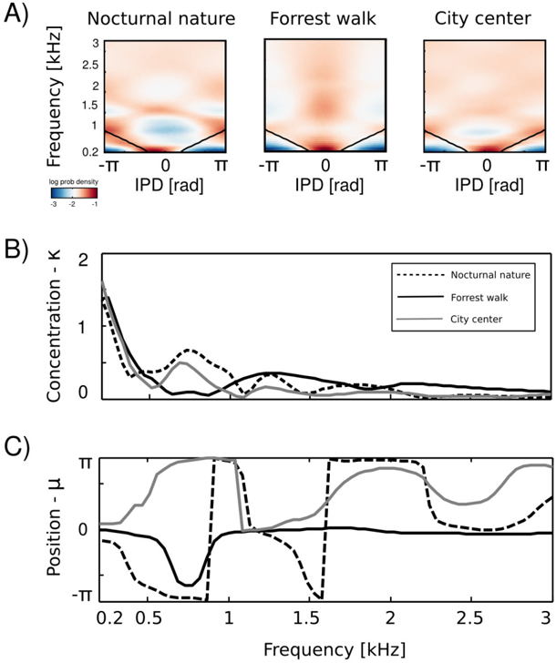
The image presents a multi-panel figure analyzing acoustic data from three different environments: "Nocturnal nature," "Forrest walk," and "City center." The figure is divided into three sections (A, B, and C). Section A displays heatmaps showing the log probability density as a function of frequency and interaural phase difference (IPD). Section B shows the concentration (kappa) as a function of frequency for each environment. Section C shows the position (mu) as a function of frequency for each environment.
### Components/Axes
**Panel A (Heatmaps):**
* **Title:** Nocturnal nature, Forrest walk, City center (one heatmap for each)
* **Y-axis:** Frequency [kHz], ranging from 0.2 to 3, with tick marks at 0.2, 1, 1.5, 2, 2.5, and 3.
* **X-axis:** IPD [rad], ranging from -π to π, with a tick mark at 0.
* **Colorbar:** "log prob density" ranging from -3 (blue) to -1 (red).
* The heatmaps are bounded by a black line forming a trapezoid shape.
**Panel B (Concentration vs. Frequency):**
* **Y-axis:** Concentration - κ, ranging from 0 to 2, with tick marks at 0, 1, and 2.
* **X-axis:** Frequency [kHz], ranging from 0.2 to 3, with tick marks at 0.2, 0.5, 1, 1.5, 2, 2.5, and 3.
* **Legend (top-right):**
* Nocturnal nature (black dashed line)
* Forrest walk (black solid line)
* City center (gray solid line)
**Panel C (Position vs. Frequency):**
* **Y-axis:** Position - μ, ranging from -π to π, with a tick mark at 0.
* **X-axis:** Frequency [kHz], ranging from 0.2 to 3, with tick marks at 0.2, 0.5, 1, 1.5, 2, 2.5, and 3.
* **Legend (same as Panel B):**
* Nocturnal nature (black dashed line)
* Forrest walk (black solid line)
* City center (gray solid line)
### Detailed Analysis
**Panel A (Heatmaps):**
* **Nocturnal nature:** A region of high probability density (red) is present around 1 kHz and 0 IPD. A region of low probability density (blue) is present around 1 kHz and +/- 1 IPD.
* **Forrest walk:** The probability density is generally higher (more red) compared to "Nocturnal nature," with a concentration around 0 IPD across all frequencies.
* **City center:** Similar to "Forrest walk," the probability density is generally high around 0 IPD across all frequencies.
**Panel B (Concentration vs. Frequency):**
* **Nocturnal nature (black dashed line):** Starts at approximately 1.8 at 0.2 kHz, decreases sharply to approximately 0.2 at 0.7 kHz, then fluctuates between 0 and 0.8 until 3 kHz.
* **Forrest walk (black solid line):** Starts at approximately 2 at 0.2 kHz, decreases sharply to approximately 0 at 0.7 kHz, then fluctuates between 0 and 0.6 until 3 kHz.
* **City center (gray solid line):** Starts at approximately 1.5 at 0.2 kHz, decreases sharply to approximately 0.1 at 0.7 kHz, then fluctuates between 0 and 0.5 until 3 kHz.
**Panel C (Position vs. Frequency):**
* **Nocturnal nature (black dashed line):** Starts at approximately -0.2 at 0.2 kHz, decreases to -π at approximately 0.7 kHz, jumps to π at 1 kHz, decreases to approximately -0.5 at 1.5 kHz, then fluctuates between -0.5 and 0 until 3 kHz.
* **Forrest walk (black solid line):** Starts at approximately 0 at 0.2 kHz, decreases to -π at approximately 0.7 kHz, jumps to 0 at 1 kHz, then remains relatively constant around 0 until 3 kHz.
* **City center (gray solid line):** Starts at approximately 0.2 at 0.2 kHz, increases to π at approximately 1 kHz, then remains relatively constant around π until 3 kHz.
### Key Observations
* The heatmaps in Panel A show distinct patterns of log probability density for each environment, suggesting differences in the acoustic characteristics.
* The concentration (κ) in Panel B is generally higher at lower frequencies for all environments.
* The position (μ) in Panel C shows distinct phase shifts around 1 kHz for all environments.
* The "City center" environment exhibits a consistently high position (μ) value across the frequency range.
### Interpretation
The data suggests that the acoustic environments have different characteristics in terms of interaural phase difference and frequency distribution. The heatmaps in Panel A provide a visual representation of these differences, while Panels B and C quantify the concentration and position of the acoustic signals as a function of frequency. The phase shifts observed around 1 kHz in Panel C may be related to specific acoustic features present in each environment. The consistently high position value for the "City center" environment could indicate a dominant sound source or a specific acoustic property of urban environments. The sharp drop in concentration for all environments around 0.7 kHz suggests a common feature or limitation in the acoustic data acquisition or processing.