## Heatmaps and Line Graphs: Spatial Audio Analysis in Different Environments
### Overview
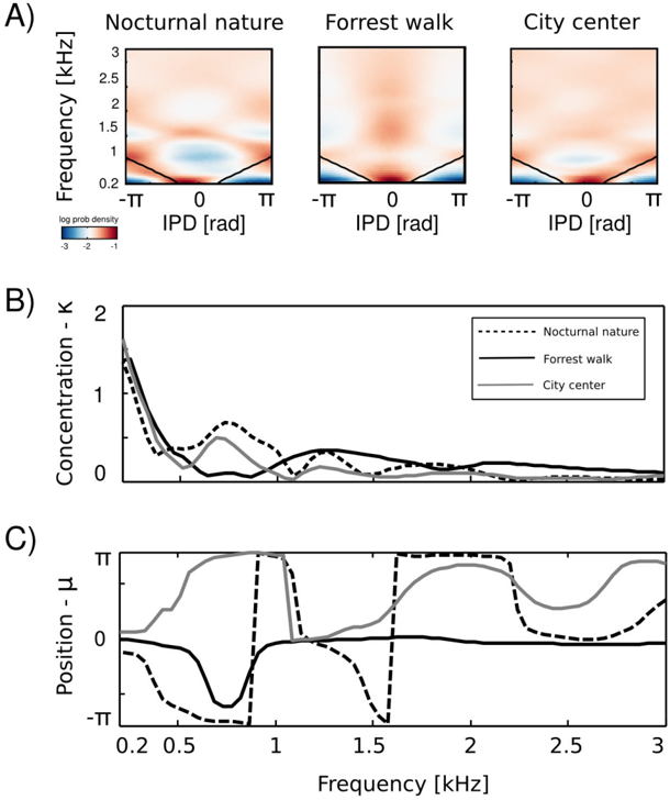
The image presents a comparative analysis of spatial audio characteristics across three environments: Nocturnal Nature, Forrest Walk, and City Center. It consists of three subplots: A) Heatmaps showing the distribution of Interaural Phase Difference (IPD) versus Frequency, B) Line graphs depicting Concentration (K) versus Frequency, and C) Line graphs showing Position (µ) versus Frequency. The data appears to be related to sound localization cues.
### Components/Axes
* **A) Heatmaps:**
* X-axis: Interaural Phase Difference (IPD) [rad], ranging from -π to π.
* Y-axis: Frequency [kHz], ranging from 0.2 to 3.
* Color Scale: Log probability density, ranging from -3 (blue) to 3 (red).
* Environments: Nocturnal Nature, Forrest Walk, City Center (displayed as separate heatmaps).
* **B) Concentration (K) vs. Frequency:**
* X-axis: Frequency [kHz], ranging from 0 to 3.
* Y-axis: Concentration - K, ranging from 0 to 2.
* Line Styles/Colors:
* Nocturnal Nature: Solid black line.
* Forrest Walk: Solid gray line.
* City Center: Dashed black line.
* **C) Position (µ) vs. Frequency:**
* X-axis: Frequency [kHz], ranging from 0 to 3.
* Y-axis: Position - µ, ranging from -π to π.
* Line Styles/Colors:
* Nocturnal Nature: Solid black line.
* Forrest Walk: Solid gray line.
* City Center: Dashed black line.
* Vertical dashed lines are present at approximately 0.2, 0.5, 1.5 and 2.5 kHz.
### Detailed Analysis or Content Details
**A) Heatmaps:**
* **Nocturnal Nature:** The heatmap shows a concentration of probability density around IPD = 0 for frequencies below 1.5 kHz. Above 1.5 kHz, the density is more dispersed, with some concentration at positive IPD values. The highest density appears to be around 0.5 kHz and IPD = 0, with a log prob density of approximately 2.5.
* **Forrest Walk:** Similar to Nocturnal Nature, the heatmap shows a concentration around IPD = 0 for lower frequencies (below 1.5 kHz). The density is more spread out at higher frequencies, with a slight bias towards positive IPD values. The highest density appears to be around 0.5 kHz and IPD = 0, with a log prob density of approximately 2.5.
* **City Center:** The heatmap is more diffuse than the other two. There is a weak concentration around IPD = 0 for lower frequencies, but the density is generally lower across the entire range. The highest density appears to be around 0.5 kHz and IPD = 0, with a log prob density of approximately 1.5.
**B) Concentration (K) vs. Frequency:**
* **Nocturnal Nature:** The line starts at approximately K = 1.8 at 0 kHz, decreases to approximately K = 0.5 at 1 kHz, and then remains relatively stable around K = 0.3 until 3 kHz.
* **Forrest Walk:** The line starts at approximately K = 1.5 at 0 kHz, decreases to approximately K = 0.4 at 1 kHz, and then remains relatively stable around K = 0.2 until 3 kHz.
* **City Center:** The line starts at approximately K = 0.8 at 0 kHz, decreases to approximately K = 0.2 at 1 kHz, and then remains relatively stable around K = 0.1 until 3 kHz.
**C) Position (µ) vs. Frequency:**
* **Nocturnal Nature:** The line oscillates around µ = 0. It has a peak at approximately µ = 0.8 at 0.5 kHz, a trough at approximately µ = -0.8 at 1 kHz, a peak at approximately µ = 0.6 at 1.5 kHz, and a trough at approximately µ = -0.4 at 2.5 kHz.
* **Forrest Walk:** The line oscillates around µ = 0, but with smaller amplitudes than Nocturnal Nature. It has a peak at approximately µ = 0.4 at 0.5 kHz, a trough at approximately µ = -0.4 at 1 kHz, a peak at approximately µ = 0.3 at 1.5 kHz, and a trough at approximately µ = -0.2 at 2.5 kHz.
* **City Center:** The line oscillates around µ = 0, but with a different phase and amplitude compared to the other two environments. It has a trough at approximately µ = -0.6 at 0.5 kHz, a peak at approximately µ = 0.6 at 1 kHz, a trough at approximately µ = -0.4 at 1.5 kHz, and a peak at approximately µ = 0.4 at 2.5 kHz.
### Key Observations
* The Nocturnal Nature and Forrest Walk environments exhibit similar patterns in both the heatmaps and line graphs, suggesting similar acoustic characteristics.
* The City Center environment shows a more diffuse IPD distribution and lower concentration values, indicating a more complex and less coherent soundscape.
* The Position (µ) curves show distinct oscillatory patterns for each environment, suggesting different spatial cues for sound localization.
* The vertical dashed lines in subplot C highlight specific frequencies where the Position (µ) curves exhibit notable changes.
### Interpretation
The data suggests that the spatial audio characteristics differ significantly between the three environments. Nocturnal Nature and Forrest Walk provide more coherent spatial cues (as indicated by the concentrated IPD distributions and higher concentration values), while the City Center environment presents a more diffuse and complex soundscape. The oscillatory patterns in the Position (µ) curves likely represent the variations in perceived sound source location as a function of frequency, and the differences between the environments suggest that the brain relies on different cues for sound localization in each setting. The lower concentration and more diffuse IPD in the City Center could be due to reflections, reverberation, and the presence of multiple sound sources. The data could be used to develop more realistic spatial audio rendering algorithms for virtual reality or augmented reality applications, tailored to specific environments. The anomalies in the City Center data suggest a more complex acoustic environment that requires more sophisticated modeling.