## Diagram: Computation Graphs and Chain-of-Thought
### Overview
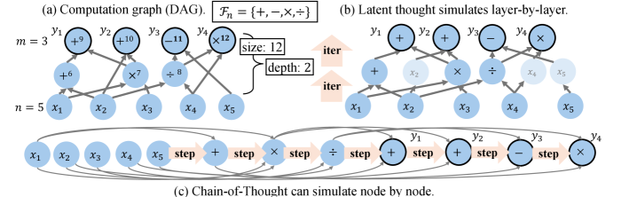
The image presents three diagrams illustrating different approaches to computation: a computation graph (DAG), a latent thought simulation, and a chain-of-thought process. The diagrams use nodes and directed edges to represent operations and data flow.
### Components/Axes
* **(a) Computation graph (DAG):**
* Title: Computation graph (DAG)
* Function Set: F\_n = {+, -, ×, ÷}
* Parameters: m = 3, n = 5
* Variables: x1, x2, x3, x4, x5, y1, y2, y3, y4
* Operations: +, ×, ÷, -
* Metadata: size: 12, depth: 2
* Nodes: Each node represents a variable or an operation. The nodes are light blue circles with a black border.
* Edges: Directed edges (gray arrows) indicate the flow of data between nodes.
* **(b) Latent thought simulates layer-by-layer:**
* Title: Latent thought simulates layer-by-layer
* Variables: x1, x2, x3, x4, x5, y1, y2, y3, y4
* Operations: +, ×, ÷, -
* Nodes: Each node represents a variable or an operation. The nodes are light blue circles with a black border. Some nodes are faded, indicating a latent or simulated state.
* Edges: Directed edges (gray arrows) indicate the flow of data between nodes.
* **(c) Chain-of-Thought:**
* Title: Chain-of-Thought can simulate node by node.
* Variables: x1, x2, x3, x4, x5, y1, y2, y3, y4
* Operations: +, ×, ÷, -
* Nodes: Each node represents a variable or an operation. The nodes are light blue circles with a black border.
* Edges: Directed edges (gray arrows) indicate the flow of data between nodes. The edges are curved to show the chain-like nature of the process.
* Steps: The process is divided into steps, indicated by light orange arrows labeled "step".
### Detailed Analysis
**(a) Computation graph (DAG):**
* The graph starts with input variables x1, x2, x3, x4, x5 at the bottom.
* These variables feed into operations: +6 (fed by x1 and x2), ×7 (fed by x2 and x3), ÷8 (fed by x3 and x4).
* The results of these operations feed into further operations: +9 (fed by +6 and ×7), +10 (fed by ×7), -11 (fed by ÷8), ×12 (fed by ÷8 and x5).
* The final results are y1 (+9), y2 (+10), y3 (-11), y4 (×12).
* The "size: 12" and "depth: 2" annotations describe the complexity of the graph.
**(b) Latent thought simulates layer-by-layer:**
* The graph starts with input variables x1, x2, x3, x4, x5 at the bottom. x4 and x5 are faded.
* These variables feed into operations: + (fed by x1 and x2), × (fed by x2 and x3), ÷ (fed by x3 and x4).
* The results of these operations feed into further operations: + (fed by + and ×), - (fed by × and ÷), × (fed by ÷ and x5).
* The final results are y1 (+), y2 (+), y3 (-), y4 (×).
**(c) Chain-of-Thought:**
* The process starts with input variables x1, x2, x3, x4, x5.
* These variables are processed sequentially through a series of operations: +, ×, ÷, +, +, -, ×.
* The results of each step are passed to the next step.
* The final results are y1 (+), y2 (+), y3 (-), y4 (×).
### Key Observations
* The computation graph (DAG) represents a parallel computation, where multiple operations can be performed simultaneously.
* The latent thought simulation shows a layer-by-layer processing of information, with some nodes being in a latent or simulated state.
* The chain-of-thought process represents a sequential computation, where each step depends on the previous step.
### Interpretation
The diagrams illustrate different approaches to computation, each with its own advantages and disadvantages. The computation graph (DAG) is efficient for parallel computation, but it can be complex to design. The latent thought simulation is useful for modeling cognitive processes, but it can be difficult to interpret. The chain-of-thought process is simple and easy to understand, but it can be slow for complex computations. The image suggests that the choice of computation approach depends on the specific problem being solved and the desired trade-offs between efficiency, interpretability, and simplicity.