## Chart: Log Probability vs. Number of Layers at Different Temperatures ### Overview The image is a scatter plot showing the relationship between the absolute value of the difference between the log base 10 of probability *P* of *AR* with *l* layers and the average log base 10 of probability *P* of *AR*, and the number of layers (*l*) for different temperatures (*T*). The plot includes data points and dashed lines representing the trend for each temperature. ### Components/Axes * **X-axis:** Number of layers, *l*. Scale ranges from 2 to 10, with integer markings. * **Y-axis:** |<log *P*_*AR*^*l*>_data - <log *P*_*AR*¹⁰>_data|. Scale ranges from 0.00 to 2.00, with markings at intervals of 0.25. * **Legend:** Located in the top-right corner, the legend maps colors to temperatures: * Blue: *T* = 0.58 * Dark Purple: *T* = 0.72 * Purple: *T* = 0.86 * Pink: *T* = 1.02 * Red-Pink: *T* = 1.41 * Orange: *T* = 1.95 * Yellow: *T* = 2.83 * **Title:** There is no explicit title, but the axes labels and legend provide context. * **Annotation:** The label "(b)" is present in the top-left corner of the plot. ### Detailed Analysis The plot shows how the absolute value of the difference between the log base 10 of probability *P* of *AR* with *l* layers and the average log base 10 of probability *P* of *AR* changes with the number of layers at different temperatures. Each temperature has a corresponding data series represented by colored dots and a dashed line. * **T = 0.58 (Blue):** Starts at approximately 2.1 at *l* = 2 and decreases rapidly, reaching approximately 0.5 at *l* = 10. * **T = 0.72 (Dark Purple):** Starts at approximately 1.9 at *l* = 2 and decreases rapidly, reaching approximately 0.3 at *l* = 10. * **T = 0.86 (Purple):** Starts at approximately 1.5 at *l* = 2 and decreases rapidly, reaching approximately 0.2 at *l* = 10. * **T = 1.02 (Pink):** Starts at approximately 1.1 at *l* = 2 and decreases rapidly, reaching approximately 0.15 at *l* = 10. * **T = 1.41 (Red-Pink):** Starts at approximately 0.5 at *l* = 2 and decreases rapidly, reaching approximately 0.05 at *l* = 10. * **T = 1.95 (Orange):** Starts at approximately 0.2 at *l* = 2 and decreases rapidly, reaching approximately 0.02 at *l* = 10. * **T = 2.83 (Yellow):** Starts at approximately 0.05 at *l* = 2 and decreases rapidly, reaching approximately 0.01 at *l* = 10. All data series show a decreasing trend as the number of layers increases. The rate of decrease appears to be higher for lower temperatures. ### Key Observations * The absolute value of the difference between the log base 10 of probability *P* of *AR* with *l* layers and the average log base 10 of probability *P* of *AR* decreases as the number of layers increases for all temperatures. * The rate of decrease is more pronounced at lower temperatures. * The curves appear to converge towards zero as the number of layers increases. * The initial values (at *l* = 2) are higher for lower temperatures. ### Interpretation The plot suggests that as the number of layers increases, the log probability of *AR* converges towards a stable value, regardless of the temperature. The convergence is faster at lower temperatures, indicating that the system reaches a more stable state with fewer layers when the temperature is lower. The higher initial values at lower temperatures suggest that the initial deviation from the average log probability is greater at lower temperatures, but this deviation is quickly reduced as the number of layers increases. The data demonstrates that the number of layers has a significant impact on the log probability of *AR*, and this impact is modulated by temperature.

## Chart: Difference in Log Probabilities vs. Number of Layers ### Overview The image presents a line chart illustrating the difference between the log probability of the area ratio (logP^l_AR) data and a reference value, plotted against the number of layers (ℓ). Multiple lines represent different values of a parameter 'T'. Error bars are present for each data point, indicating the uncertainty in the measurements. ### Components/Axes * **X-axis:** Number of layers (ℓ), ranging from approximately 2 to 10. Labeled as "Number of layers, ℓ". * **Y-axis:** Difference in log probabilities: ⟨logP^l_AR data - ⟨logP^l_AR⟩data⟩, ranging from approximately 0 to 2. Labeled as "⟨logP^l_AR data - ⟨logP^l_AR⟩data⟩". * **Legend:** Located in the top-right corner, listing the values of 'T' corresponding to each line: * T = 0.58 (Dark Blue) * T = 0.72 (Medium Blue) * T = 0.86 (Purple) * T = 1.02 (Magenta) * T = 1.41 (Red) * T = 1.95 (Orange) * T = 2.83 (Yellow) * **Title:** "(b)" located in the top-left corner. ### Detailed Analysis The chart displays seven distinct lines, each representing a different value of 'T'. All lines exhibit a decreasing trend as the number of layers (ℓ) increases. The initial values and rates of decrease vary significantly between the lines. * **T = 0.58 (Dark Blue):** The line starts at approximately 1.85 at ℓ = 2 and decreases rapidly, approaching 0 around ℓ = 8. Error bars are visible and relatively large at lower ℓ values, decreasing as ℓ increases. * **T = 0.72 (Medium Blue):** Starts at approximately 1.55 at ℓ = 2, decreasing more slowly than T = 0.58. Approaches 0 around ℓ = 9. Error bars are similar in size to T = 0.58. * **T = 0.86 (Purple):** Starts at approximately 1.2 at ℓ = 2, decreasing at a rate between T = 0.72 and T = 1.02. Approaches 0 around ℓ = 9. Error bars are similar in size to T = 0.58. * **T = 1.02 (Magenta):** Starts at approximately 0.85 at ℓ = 2, decreasing at a slower rate than the previous lines. Approaches 0 around ℓ = 9. Error bars are similar in size to T = 0.58. * **T = 1.41 (Red):** Starts at approximately 0.3 at ℓ = 2, and decreases slowly. Approaches 0 around ℓ = 6. Error bars are relatively small. * **T = 1.95 (Orange):** Starts at approximately 0.15 at ℓ = 2, and decreases very slowly. Approaches 0 around ℓ = 6. Error bars are relatively small. * **T = 2.83 (Yellow):** Starts at approximately 0.05 at ℓ = 2, and remains close to 0 throughout the plotted range. Error bars are relatively small. ### Key Observations * The difference in log probabilities decreases with increasing number of layers for all values of 'T'. * Lower values of 'T' (0.58, 0.72, 0.86, 1.02) exhibit a more significant initial difference and a more pronounced decrease compared to higher values of 'T' (1.41, 1.95, 2.83). * The error bars suggest greater uncertainty in the measurements for lower values of 'T' and at smaller values of ℓ. * The lines for T = 1.95 and T = 2.83 are consistently close to zero, indicating a minimal difference in log probabilities for these values of 'T'. ### Interpretation This chart likely represents the convergence of a model or algorithm as the number of layers increases. The parameter 'T' could represent a control parameter or a characteristic of the input data. The decreasing trend suggests that as the number of layers increases, the model's output becomes more consistent or approaches a stable state. The different lines for different values of 'T' indicate that the convergence rate and initial difference are sensitive to the value of 'T'. The larger error bars for lower 'T' values suggest that the model is more sensitive to variations in the input data or initial conditions when 'T' is small. The fact that the lines for higher 'T' values are closer to zero and have smaller error bars suggests that the model is more robust and converges more quickly for these values of 'T'. The chart demonstrates a clear relationship between the parameter 'T', the number of layers, and the difference in log probabilities, providing insights into the behavior and convergence properties of the underlying model.

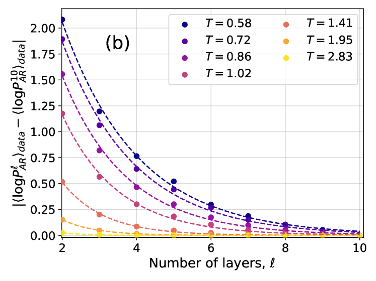
\n ## Line Graph: Decay of Logarithmic Difference vs. Number of Layers ### Overview The image is a scientific line graph, labeled "(b)" in its top-left corner, plotting the absolute difference between two logarithmic quantities against the number of layers, ℓ. The graph displays seven distinct data series, each corresponding to a different value of a parameter `T`. All series show a decaying trend as the number of layers increases. ### Components/Axes * **Chart Label:** "(b)" located in the top-left quadrant of the plot area. * **X-Axis:** * **Title:** "Number of layers, ℓ" * **Scale:** Linear, ranging from 2 to 10. * **Major Tick Marks:** At integers 2, 4, 6, 8, 10. * **Y-Axis:** * **Title:** `| (log P_AR^ℓ)_data - (log P_AR^10)_data |` * **Scale:** Linear, ranging from 0.00 to 2.00. * **Major Tick Marks:** At intervals of 0.25 (0.00, 0.25, 0.50, ..., 2.00). * **Legend:** Positioned in the top-right corner of the plot area. It contains seven entries, each pairing a colored circle marker with a `T` value. * **Entries (from top to bottom):** 1. Dark Blue Circle: `T = 0.58` 2. Purple Circle: `T = 0.72` 3. Magenta Circle: `T = 0.86` 4. Pink Circle: `T = 1.02` 5. Salmon/Light Red Circle: `T = 1.41` 6. Orange Circle: `T = 1.95` 7. Yellow Circle: `T = 2.83` ### Detailed Analysis The graph plots the convergence of a quantity `log P_AR^ℓ` (for ℓ layers) towards its value at 10 layers (`log P_AR^10`). The y-axis measures the absolute difference from this reference point. **Trend Verification & Data Points (Approximate):** For each series, the value decreases monotonically as ℓ increases from 2 to 10. The decay is initially rapid and then asymptotes towards zero. 1. **T = 0.58 (Dark Blue):** Starts highest. At ℓ=2, y ≈ 2.05. Decays to y ≈ 0.05 at ℓ=10. 2. **T = 0.72 (Purple):** At ℓ=2, y ≈ 1.90. Decays to y ≈ 0.04 at ℓ=10. 3. **T = 0.86 (Magenta):** At ℓ=2, y ≈ 1.55. Decays to y ≈ 0.03 at ℓ=10. 4. **T = 1.02 (Pink):** At ℓ=2, y ≈ 1.20. Decays to y ≈ 0.02 at ℓ=10. 5. **T = 1.41 (Salmon):** At ℓ=2, y ≈ 0.52. Decays to y ≈ 0.01 at ℓ=10. 6. **T = 1.95 (Orange):** At ℓ=2, y ≈ 0.15. Decays to y ≈ 0.005 at ℓ=10. 7. **T = 2.83 (Yellow):** Starts lowest. At ℓ=2, y ≈ 0.03. Decays to nearly 0.00 at ℓ=10. **Key Observation:** The initial value (at ℓ=2) and the rate of decay are strongly dependent on the parameter `T`. Lower `T` values result in a larger initial difference and a slower convergence to the 10-layer value. ### Key Observations * **Systematic Ordering:** The curves are perfectly ordered by `T` value. At any given layer ℓ, a lower `T` corresponds to a higher y-value. * **Convergence:** All series appear to converge to a difference of approximately zero by ℓ=10, which is expected as the y-axis measures the difference from the value at ℓ=10 itself. * **Shape:** The decay for each series follows a similar convex, decreasing curve, suggesting an exponential or power-law relationship between the difference and the number of layers. ### Interpretation This graph demonstrates the convergence behavior of a model or calculation (`P_AR`) as its depth (number of layers, ℓ) increases. The quantity `log P_AR^ℓ` is being compared to its "converged" value at 10 layers. * **What the data suggests:** The parameter `T` controls the difficulty or scale of the convergence. Lower `T` values represent a scenario where the model's output at shallow depths (low ℓ) is very different from its deep (ℓ=10) output, requiring many more layers to stabilize. Higher `T` values represent an "easier" scenario where the model's output is already close to its final value even with very few layers. * **Relationship between elements:** The x-axis (model depth) is the independent variable driving convergence. The y-axis (log difference) is the dependent measure of error or change. The legend (`T`) is a control parameter that modulates the relationship between depth and convergence speed. * **Notable implication:** The plot provides a quantitative way to assess how many layers are needed for the model's output to become stable for a given `T`. For `T=2.83`, 2-4 layers may suffice, while for `T=0.58`, even 8 layers show a non-negligible difference from the 10-layer result. This is critical for understanding computational efficiency and model design trade-offs.

## Line Graph: Relationship Between Number of Layers and Log P_AR^10 Difference ### Overview The graph illustrates the relationship between the number of layers (ℓ) and the absolute difference in logarithmic values of ⟨log P_AR^10⟩_data for various temperature (T) conditions. Six distinct data series are plotted, each corresponding to a specific T value, with trends showing how the difference evolves as the number of layers increases from 2 to 10. ### Components/Axes - **X-axis**: "Number of layers, ℓ" (integer values from 2 to 10). - **Y-axis**: "|⟨log P_AR^10⟩_data − ⟨log P_AR^10⟩_data|" (logarithmic scale, ranging from 0.00 to 2.00). - **Legend**: Located in the top-right corner, mapping six T values to colors: - **T = 0.58** (dark blue, solid circles) - **T = 0.72** (purple, solid circles) - **T = 0.86** (magenta, solid circles) - **T = 1.02** (pink, solid circles) - **T = 1.41** (orange, solid circles) - **T = 1.95** (yellow, solid circles) - **T = 2.83** (red, solid circles) - **Line Style**: All lines are dashed, with markers (circles) at each data point. ### Detailed Analysis 1. **T = 0.58 (dark blue)**: - Starts at ~2.00 for ℓ = 2, decreasing sharply to ~0.05 by ℓ = 10. - Steepest decline among all series. 2. **T = 0.72 (purple)**: - Begins at ~1.80 for ℓ = 2, dropping to ~0.10 by ℓ = 10. - Intermediate slope compared to other series. 3. **T = 0.86 (magenta)**: - Initial value ~1.60 at ℓ = 2, decreasing to ~0.15 at ℓ = 10. - Moderate decline rate. 4. **T = 1.02 (pink)**: - Starts at ~1.40 for ℓ = 2, falling to ~0.20 at ℓ = 10. - Slower decline than lower T values. 5. **T = 1.41 (orange)**: - Begins at ~0.50 for ℓ = 2, dropping to ~0.05 at ℓ = 10. - Shallow slope, minimal change across layers. 6. **T = 1.95 (yellow)**: - Starts at ~0.30 for ℓ = 2, decreasing to ~0.02 at ℓ = 10. - Very gradual decline. 7. **T = 2.83 (red)**: - Initial value ~0.10 at ℓ = 2, remaining near 0.00 for ℓ ≥ 4. - Near-zero difference after ℓ = 4. ### Key Observations - **Inverse Relationship**: Higher T values correlate with smaller absolute differences in ⟨log P_AR^10⟩_data. - **Convergence**: All series approach zero as ℓ increases, with higher T values stabilizing faster. - **Layer Sensitivity**: Lower T values (e.g., 0.58) exhibit stronger dependence on layer count, while higher T values (e.g., 2.83) show minimal layer-dependent variation. - **Data Point Consistency**: All markers align precisely with their respective legend colors, confirming accurate series identification. ### Interpretation The data suggests that temperature (T) modulates the sensitivity of ⟨log P_AR^10⟩_data to the number of layers. Lower T values amplify layer-dependent variations, while higher T values suppress these effects, potentially indicating a saturation or equilibrium state. The convergence of all series toward zero at higher layers implies that beyond a critical layer count (ℓ > 8), the system reaches a stable configuration where T has negligible impact. This could reflect a phase transition or critical threshold in the modeled system, where increasing layers homogenize the logarithmic differences regardless of T. The stark contrast between T = 0.58 (high sensitivity) and T = 2.83 (near-zero sensitivity) highlights T as a critical parameter governing system behavior.