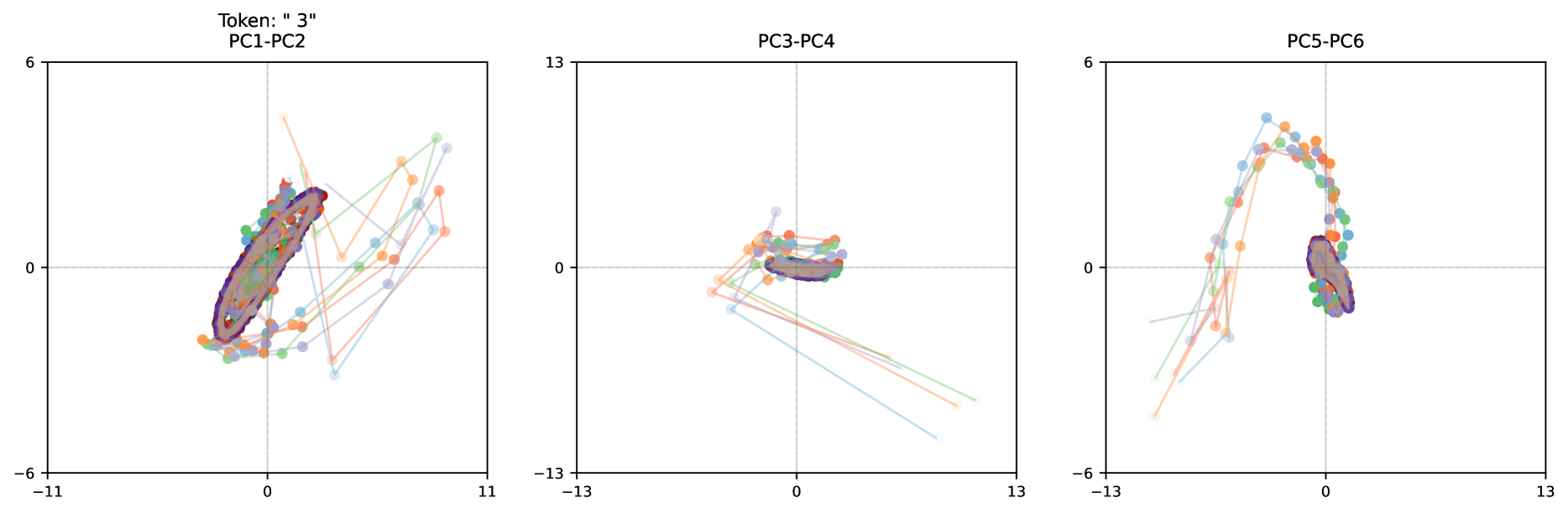
## Scatter Plots: Token "3" Analysis Across Principal Component Pairs ### Overview Three scatter plots visualize the distribution of data points across different principal component (PC) pairs, labeled as PC1-PC2, PC3-PC4, and PC5-PC6. Each plot includes colored data points and connecting lines, with axis ranges varying significantly between plots. The title "Token: '3'" suggests the data relates to a specific identifier or category. --- ### Components/Axes 1. **PC1-PC2 Plot**: - **X-axis (PC1)**: Ranges from -11 to 11. - **Y-axis (PC2)**: Ranges from -6 to 6. - **Legend**: Not visible in the image. - **Data Points**: Colored dots (purple, green, orange, blue, red) clustered in the lower-left quadrant, with sparse points extending to the upper-right. 2. **PC3-PC4 Plot**: - **X-axis (PC3)**: Ranges from -13 to 13. - **Y-axis (PC4)**: Ranges from -13 to 13. - **Legend**: Not visible in the image. - **Data Points**: Central cluster near the origin, with lines radiating outward to peripheral points. 3. **PC5-PC6 Plot**: - **X-axis (PC5)**: Ranges from -13 to 13. - **Y-axis (PC6)**: Ranges from -6 to 6. - **Legend**: Not visible in the image. - **Data Points**: Curved trajectory of points forming an arc from lower-left to upper-right, with a dense cluster in the lower-right quadrant. --- ### Detailed Analysis #### PC1-PC2 Plot - **Trend**: A dense cluster of points dominates the lower-left quadrant (PC1 ≈ -5 to -1, PC2 ≈ -3 to 0), with a smaller cluster in the upper-right (PC1 ≈ 2 to 5, PC2 ≈ 2 to 5). Lines connect points in a non-linear, scattered pattern. - **Key Data Points**: - Purple cluster: Centered at (-4, -2). - Green cluster: Centered at (3, 3). - Orange points: Scattered along PC1 ≈ 0 to 3, PC2 ≈ -2 to 1. #### PC3-PC4 Plot - **Trend**: A central cluster near the origin (PC3 ≈ -2 to 2, PC4 ≈ -2 to 2) with lines extending to peripheral points in all quadrants. - **Key Data Points**: - Central cluster: Mixed colors (purple, green, orange) concentrated near (0, 0). - Peripheral points: Blue and red dots at extremes (e.g., PC3 ≈ ±10, PC4 ≈ ±5). #### PC5-PC6 Plot - **Trend**: A curved trajectory of points forms an arc from lower-left (PC5 ≈ -8, PC6 ≈ -4) to upper-right (PC5 ≈ 8, PC6 ≈ 4), with a dense cluster in the lower-right (PC5 ≈ 2 to 5, PC6 ≈ -2 to 0). - **Key Data Points**: - Arc: Points transition from purple (lower-left) to green/orange (upper-right). - Lower-right cluster: High density of green and orange points. --- ### Key Observations 1. **Clustered Distributions**: All plots show distinct groupings, suggesting latent categories or hierarchical structures in the data. 2. **Line Connections**: Lines in PC1-PC2 and PC3-PC4 plots may represent transitions or relationships between data points (e.g., temporal or causal links). 3. **Axis Scaling**: PC3-PC4 and PC5-PC6 plots use larger axis ranges, indicating greater variability in those components. 4. **Missing Legend**: Color coding cannot be definitively interpreted without a legend, limiting categorical analysis. --- ### Interpretation - **Principal Component Analysis (PCA)**: The plots likely represent PCA results, where each axis captures maximal variance in the data. The token "3" may denote a subset of data (e.g., a specific class or time series). - **Dimensionality Reduction**: The separation of PC pairs (e.g., PC1-PC2 vs. PC5-PC6) suggests that earlier components capture more significant variance, while later components reveal finer-grained patterns. - **Anomalies**: The curved trajectory in PC5-PC6 could indicate a cyclical or nonlinear relationship in the data, while the central cluster in PC3-PC4 might represent a baseline or control group. - **Practical Implications**: These plots could be used for feature selection, anomaly detection, or clustering in high-dimensional datasets (e.g., NLP, genomics, or image processing). --- ### Limitations - **Lack of Legend**: Color meanings (e.g., categories, classes) are unspecified. - **No Context**: The purpose of "Token: '3'" and the dataset’s domain are unclear. - **Axis Ranges**: Varying scales complicate direct comparisons between plots.