\n
## Q-Q Plot: w(n) vs. Normal Distribution
### Overview
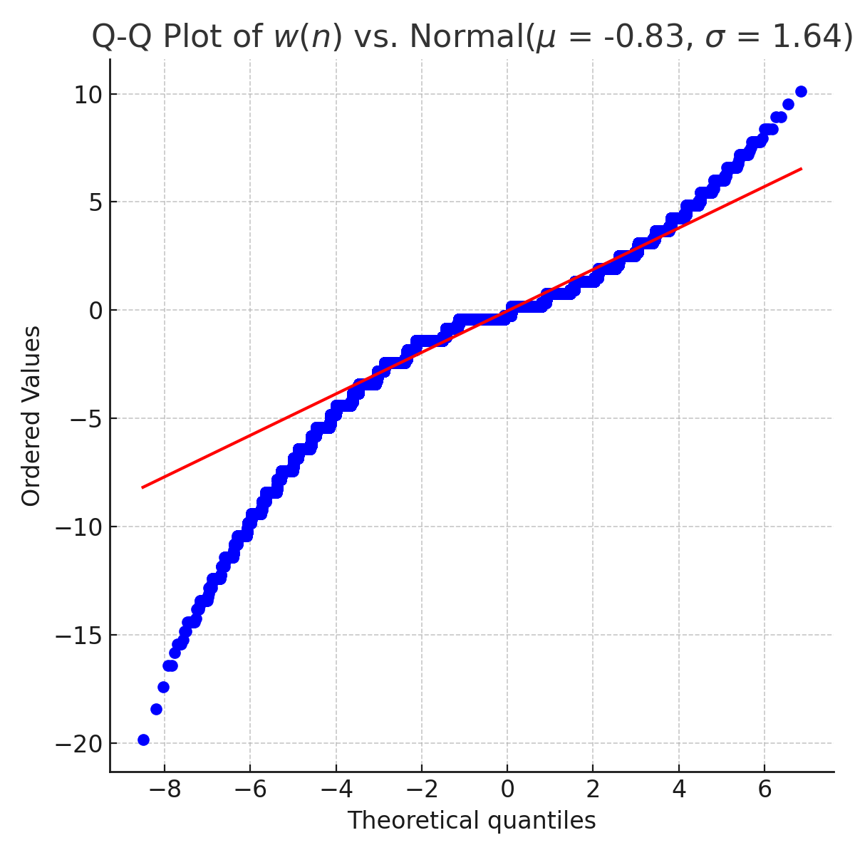
This image displays a Quantile-Quantile (Q-Q) plot comparing the distribution of `w(n)` to a normal distribution with a mean (μ) of -0.83 and a standard deviation (σ) of 1.64. The plot assesses how well the quantiles of `w(n)` align with the quantiles of the specified normal distribution.
### Components/Axes
* **Title:** "Q-Q Plot of w(n) vs. Normal(μ = -0.83, σ = 1.64)" - Located at the top-center of the image.
* **X-axis:** "Theoretical quantiles" - Ranges approximately from -8 to 6.
* **Y-axis:** "Ordered Values" - Ranges approximately from -20 to 10.
* **Data Points:** Blue dots representing the ordered values of `w(n)`.
* **Reference Line:** A red line representing the expected quantiles for a perfect normal distribution.
### Detailed Analysis
The plot shows a series of blue data points plotted against the theoretical quantiles. A red line is overlaid to represent the expected distribution if `w(n)` were perfectly normally distributed.
* **Lower Tail:** From approximately (-8, -20) to (-4, -5), the blue points deviate noticeably *below* the red line. This indicates that the lower tail of `w(n)` is heavier than the lower tail of the normal distribution.
* **Middle Section:** From approximately (-4, -5) to (2, 0), the blue points generally follow the red line, but with some scatter.
* **Upper Tail:** From approximately (2, 0) to (6, 10), the blue points closely align with the red line, suggesting the upper tail of `w(n)` is well-represented by the normal distribution.
Let's approximate some data points:
* (-8, -20): A blue point is located here.
* (-6, -14): A blue point is located here.
* (-4, -8): A blue point is located here.
* (-2, -2): A blue point is located here.
* (0, 2): A blue point is located here.
* (2, 5): A blue point is located here.
* (4, 8): A blue point is located here.
* (6, 10): A blue point is located here.
The red line can be approximated as:
* (-8, -8)
* (-4, -4)
* (0, 0)
* (4, 4)
* (6, 6)
### Key Observations
* The most significant deviation from normality occurs in the lower tail of the distribution.
* The upper tail appears to be reasonably well-aligned with the normal distribution.
* The plot suggests that `w(n)` is not perfectly normally distributed, primarily due to the heavier lower tail.
### Interpretation
The Q-Q plot indicates that the distribution of `w(n)` is not perfectly normal. The deviation in the lower tail suggests that `w(n)` has more extreme negative values than would be expected from a normal distribution with the given mean and standard deviation. This could be due to several factors, such as skewness, outliers, or a different underlying distribution altogether. The relatively good alignment in the upper tail suggests that the positive values of `w(n)` are reasonably well-represented by the normal distribution.
The plot is a diagnostic tool for assessing the normality assumption, which is important for many statistical tests and models. The observed deviation suggests that caution should be exercised when applying methods that rely on the normality assumption to `w(n)`. Further investigation into the nature of the lower tail deviation might be warranted to understand the underlying process generating the data.