## Q-Q Plot: w(n) vs. Normal(μ = -0.83, σ = 1.64)
### Overview
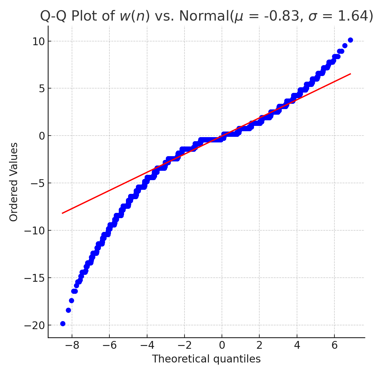
The image is a Q-Q (quantile-quantile) plot comparing ordered values of a dataset (`w(n)`) against theoretical quantiles from a normal distribution with mean μ = -0.83 and standard deviation σ = 1.64. The plot includes a red reference line (45-degree line) and blue data points representing the dataset.
---
### Components/Axes
- **X-axis**: "Theoretical quantiles" (range: -8 to 6, increments of 2).
- **Y-axis**: "Ordered Values" (range: -20 to 10, increments of 5).
- **Legend**:
- Red: "Reference line" (45-degree line).
- Blue: "Ordered Values" (data points).
- **Grid**: Dotted gray lines for reference.
---
### Detailed Analysis
1. **Reference Line (Red)**:
- A straight diagonal line from bottom-left to top-right, representing perfect agreement between theoretical and observed quantiles.
- Equation: y = x (approximate).
2. **Data Points (Blue Dots)**:
- **Left Tail (x < -2)**:
- Points cluster below the reference line, indicating observed values are smaller than theoretical quantiles.
- Example: At x ≈ -8, y ≈ -20 (observed value is ~12 units lower than theoretical).
- **Center (x ≈ -2 to 2)**:
- Points align closely with the reference line, suggesting agreement in central quantiles.
- Example: At x ≈ 0, y ≈ 0.
- **Right Tail (x > 2)**:
- Points diverge above the reference line, indicating observed values are larger than theoretical quantiles.
- Example: At x ≈ 6, y ≈ 10 (observed value is ~4 units higher than theoretical).
3. **Distribution Shape**:
- The dataset exhibits **asymmetry**:
- Left tail (negative x) is lighter (points below the line).
- Right tail (positive x) is heavier (points above the line).
- This suggests the dataset may have **leptokurtic (fat-tailed) behavior** on the right and **platykurtic (thin-tailed) behavior** on the left compared to the assumed normal distribution.
---
### Key Observations
- **Deviations at Extremes**:
- Left tail (x < -4): Observed values are systematically lower than theoretical.
- Right tail (x > 2): Observed values are systematically higher than theoretical.
- **Central Agreement**:
- Quantiles near the mean (x ≈ -2 to 2) align well with the normal distribution.
- **Outliers**:
- No extreme outliers visible, but the right tail shows mild skewness.
---
### Interpretation
The Q-Q plot reveals that the dataset `w(n)` does not fully conform to the assumed normal distribution (μ = -0.83, σ = 1.64). The deviations at the extremes suggest:
1. **Right-Skewness**: The right tail of the dataset is heavier than the normal distribution, potentially indicating the presence of mild outliers or a non-normal distribution with positive kurtosis.
2. **Left-Skewness**: The left tail is lighter, possibly due to truncation or a bounded lower limit in the data.
3. **Parameter Mismatch**: The theoretical normal distribution parameters (μ, σ) may not accurately represent the dataset’s central tendency and spread, as the central quantiles align well, but the tails do not.
This analysis implies that statistical methods assuming normality (e.g., t-tests, ANOVA) may be less reliable for this dataset, particularly for inference involving tail behavior. Further investigation into alternative distributions (e.g., log-normal, skewed normal) or robust statistical methods is warranted.