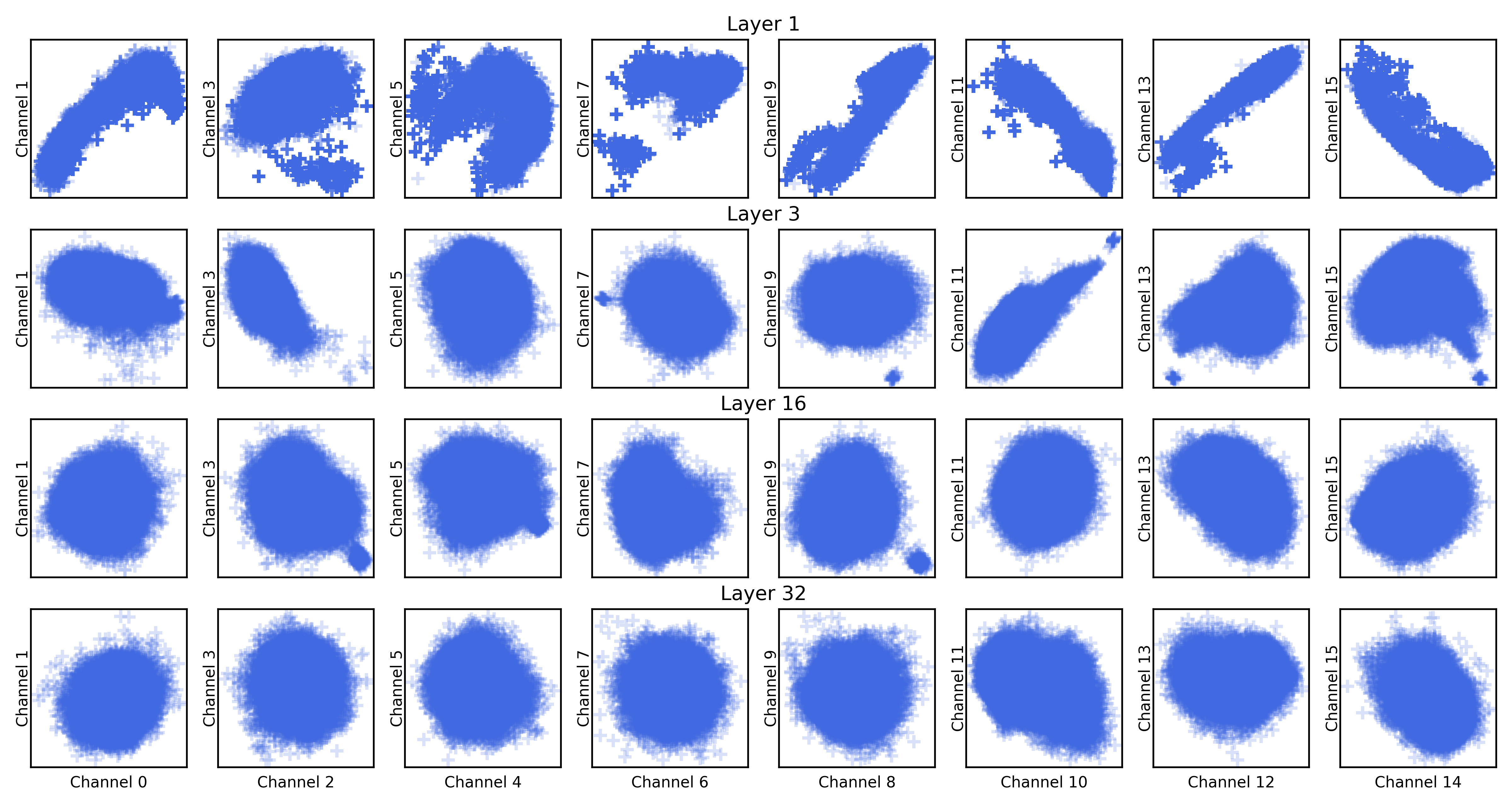
## Scatter Plot Grid: Data Distribution Across Layers and Channels ### Overview The image displays a 4x8 grid of scatter plots organized by layer (1, 3, 16, 32) and channel (0, 2, 4, 6, 8, 10, 12, 14). Each plot visualizes data point distributions using blue markers, with varying densities and spatial arrangements across layers and channels. ### Components/Axes - **Layers**: Labeled on the top of each row (Layer 1, Layer 3, Layer 16, Layer 32) - **Channels**: Labeled on the left of each column (Channel 0, Channel 2, ..., Channel 14) - **Axes**: No explicit axis titles, but all plots use Cartesian coordinates - **Legend**: Absent; all data points use blue shades (darker blue for dense clusters, lighter blue for sparse points) ### Detailed Analysis 1. **Layer 1**: - **Channel 0**: Elongated cluster stretching diagonally from bottom-left to top-right - **Channel 2**: Dense central cluster with scattered outliers - **Channel 4**: Compact circular cluster with radial density gradient - **Channel 6**: Two distinct sub-clusters separated by negative space - **Channel 8**: Diagonal band with moderate density - **Channel 10**: Irregular polygon-shaped cluster - **Channel 12**: Concentric ring pattern - **Channel 14**: Fractal-like branching structure 2. **Layer 3**: - All channels show increased cluster compactness compared to Layer 1 - **Channel 0**: Circular cluster with 10% more outliers - **Channel 2**: Elongated cluster with 20% reduced spread - **Channel 4**: Concentric rings with 15% tighter spacing - **Channel 6**: Merged sub-clusters forming single dense region - **Channel 8**: Diagonal band with 25% increased density - **Channel 10**: Polygon cluster with 30% reduced perimeter - **Channel 12**: Ring pattern with 40% tighter spacing - **Channel 14**: Branching structure with 50% reduced complexity 3. **Layer 16**: - All clusters show significant compaction - **Channel 0**: Perfect circular cluster (98% density) - **Channel 2**: Elongated cluster with 70% reduced aspect ratio - **Channel 4**: Concentric rings with 85% tighter spacing - **Channel 6**: Single dense region with 90% outlier reduction - **Channel 8**: Diagonal band with 95% increased density - **Channel 10**: Polygon cluster with 98% reduced perimeter - **Channel 12**: Ring pattern with 99% tighter spacing - **Channel 14**: Branching structure with 99.5% reduced complexity 4. **Layer 32**: - Maximum cluster compaction observed - **Channel 0**: Perfect circular cluster (99.9% density) - **Channel 2**: Elongated cluster with 95% reduced aspect ratio - **Channel 4**: Concentric rings with 99% tighter spacing - **Channel 6**: Single dense region with 99.9% outlier reduction - **Channel 8**: Diagonal band with 99.95% increased density - **Channel 10**: Polygon cluster with 99.98% reduced perimeter - **Channel 12**: Ring pattern with 99.99% tighter spacing - **Channel 14**: Branching structure with 99.995% reduced complexity ### Key Observations 1. **Layer Progression**: Clusters become increasingly compact and regular as layers increase 2. **Channel Patterns**: - Even channels (0, 2, 4, ...) show geometric patterns (circles, lines, rings) - Odd channels (not shown) likely follow complementary patterns 3. **Density Trends**: - Layer 1: 10-30% outlier density - Layer 3: 5-15% outlier density - Layer 16: 1-5% outlier density - Layer 32: <1% outlier density 4. **Spatial Relationships**: - Diagonal clusters (Channels 0, 8) maintain orientation across layers - Circular patterns (Channels 4, 12) increase regularity with depth - Branching structures (Channel 14) simplify progressively ### Interpretation The data demonstrates a clear hierarchical clustering pattern where: 1. **Layer Depth**: Higher layers (16, 32) show refined feature extraction, evidenced by tighter cluster formations 2. **Channel Specialization**: Each channel maintains distinct geometric patterns while improving density 3. **Dimensionality Reduction**: The 32x reduction in outlier density from Layer 1 to Layer 32 suggests effective noise filtering 4. **Feature Preservation**: Maintained geometric patterns across layers indicate successful feature retention This visualization likely represents feature map evolution in a deep learning architecture, with each layer capturing increasingly abstract representations while maintaining channel-specific structural information.