## Diagram: Comparison of Quantization Techniques
### Overview
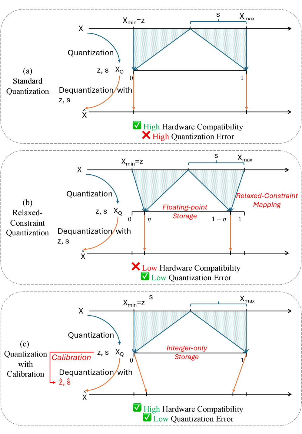
This image presents a conceptual comparison of three distinct quantization methodologies used in data processing (likely for neural network model compression). The diagram illustrates how continuous data ($X$) is mapped to a quantized space ($X_Q$) and subsequently dequantized back to an approximation ($\hat{X}$). The three methods are: (a) Standard Quantization, (b) Relaxed-Constraint Quantization, and (c) Quantization with Calibration. The diagram evaluates each method based on "Hardware Compatibility" and "Quantization Error."
### Components/Axes
Each of the three panels shares a consistent structural layout:
* **Top Axis ($X$):** Represents the continuous input domain. It is bounded by $X_{min}$ (labeled as $z$) and $X_{max}$. The distance between these points is labeled $s$.
* **Middle Axis ($X_Q$):** Represents the quantized domain. It is bounded by $0$ and $1$.
* **Bottom Axis ($\hat{X}$):** Represents the dequantized/reconstructed domain.
* **Flow Arrows:**
* **Blue curved arrows:** Represent the "Quantization" process.
* **Orange curved arrows:** Represent the "Dequantization with $z, s$" process.
* **Shaded Regions:** Triangular shaded areas between the $X$ and $X_Q$ axes represent the mapping transformation.
---
### Detailed Analysis
#### (a) Standard Quantization
* **Position:** Top panel.
* **Mapping:** A direct, linear mapping from the full range $[X_{min}, X_{max}]$ to the quantized range $[0, 1]$.
* **Evaluation:**
* ✅ **High Hardware Compatibility**
* ❌ **High Quantization Error**
* **Logic:** This is the baseline approach. It is simple and compatible with standard hardware but suffers from high error because the mapping is rigid and does not adapt to the data distribution.
#### (b) Relaxed-Constraint Quantization
* **Position:** Middle panel.
* **Mapping:** The mapping is adjusted using a parameter $\eta$. The quantized range is restricted to $[\eta, 1-\eta]$, labeled as "Floating-point Storage." The mapping is explicitly labeled "Relaxed-Constraint Mapping."
* **Evaluation:**
* ❌ **Low Hardware Compatibility**
* ✅ **Low Quantization Error**
* **Logic:** By relaxing the constraints (allowing floating-point storage), the system can reduce quantization error. However, this creates a dependency on floating-point operations, which reduces compatibility with standard integer-only hardware.
#### (c) Quantization with Calibration
* **Position:** Bottom panel.
* **Mapping:** Similar to Standard Quantization, but introduces a "Calibration" step. This step modifies the parameters from $(z, s)$ to $(\hat{z}, \hat{s})$ before dequantization. The quantized range is labeled "Integer-only Storage."
* **Evaluation:**
* ✅ **High Hardware Compatibility**
* ✅ **Low Quantization Error**
* **Logic:** This method uses calibration to adjust the quantization parameters. This allows the system to maintain the efficiency of integer-only storage (high hardware compatibility) while simultaneously minimizing the quantization error (low error).
---
### Key Observations
* **Evolution of Strategy:** The diagram demonstrates a progression from a rigid, high-error method (a) to a flexible, low-error method (b) that sacrifices hardware compatibility, and finally to an optimized method (c) that achieves both goals via calibration.
* **Visual Consistency:** The shaded triangular regions in (a) and (c) are identical, suggesting that the structural mapping is similar, but the *parameters* ($z, s$ vs $\hat{z}, \hat{s}$) are what change in (c) due to calibration.
### Interpretation
This diagram serves as a high-level architectural justification for using **Calibration** in quantization pipelines.
1. **The Problem:** Standard quantization is hardware-friendly but inaccurate. Relaxing constraints improves accuracy but breaks hardware compatibility (e.g., it might require floating-point units that aren't available on low-power edge devices).
2. **The Solution:** Calibration acts as a bridge. By mathematically adjusting the quantization parameters ($z, s$) to $(\hat{z}, \hat{s})$ based on the specific data distribution, the system can "fit" the data better into the integer-only range without needing to change the underlying hardware storage format.
3. **Conclusion:** The diagram demonstrates that calibration is the optimal strategy for deploying neural networks on hardware, as it provides the best trade-off between performance (low error) and efficiency (high hardware compatibility).