## Line Graph: Relationship Between Processors and Time Components
### Overview
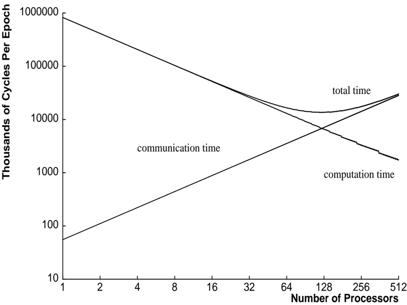
The graph illustrates the relationship between the number of processors and three time components: communication time, computation time, and total time. It uses a logarithmic scale for the y-axis (Thousands of Cycles Per Epoch) and a linear scale for the x-axis (Number of Processors). Three lines are plotted: a decreasing line for communication time, an increasing line for computation time, and a combined curve for total time.
### Components/Axes
- **Y-Axis**: "Thousands of Cycles Per Epoch" (logarithmic scale: 10, 100, 1,000, 10,000, 100,000, 1,000,000).
- **X-Axis**: "Number of Processors" (linear scale: 1, 2, 4, 8, 16, 32, 64, 128, 256, 512).
- **Legend**:
- **Communication Time**: Straight line (dark gray).
- **Computation Time**: Straight line (black).
- **Total Time**: Curved line (black, overlapping with computation time at higher processor counts).
### Detailed Analysis
1. **Communication Time**:
- Starts at ~100,000 cycles per epoch at 1 processor.
- Decreases linearly as processors increase.
- At 512 processors, approaches ~10 cycles per epoch.
2. **Computation Time**:
- Starts at ~10 cycles per epoch at 1 processor.
- Increases linearly as processors increase.
- At 512 processors, reaches ~100,000 cycles per epoch.
3. **Total Time**:
- Combines communication and computation time.
- Initially decreases sharply (dominated by communication time reduction).
- Reaches a minimum at ~32 processors (~10,000 cycles per epoch).
- Increases again beyond 32 processors (dominated by computation time growth).
### Key Observations
- **Intersection Point**: Communication and computation times cross at ~32 processors, where total time is minimized.
- **Scaling Behavior**:
- Communication time scales inversely with processors (ideal parallelization).
- Computation time scales directly with processors (potential overhead or inefficiency).
- **Total Time U-Shaped Curve**: Reflects diminishing returns after ~32 processors.
### Interpretation
The graph demonstrates a classic trade-off in parallel computing:
- **Optimal Processor Count**: ~32 processors minimize total time by balancing communication and computation overhead.
- **Beyond Optimal**: Adding more processors increases computation time disproportionately, negating communication gains.
- **Implications**: Highlights the importance of workload distribution and system architecture in parallel systems. The linear scaling of computation time suggests potential bottlenecks (e.g., Amdahl's Law limitations).