TECHNICAL ASSET FINGERPRINT
355b32440de9e04f52b12249
Click to view fullscreen
Press ESC or click to close
FOUND IN PAPERS
EXPERT: healer-alpha-free VERSION 1
RUNTIME: free/openrouter/healer-alpha
INTEL_VERIFIED
\n
## Multi-Panel Technical Figure: Curriculum Learning Analysis
### Overview
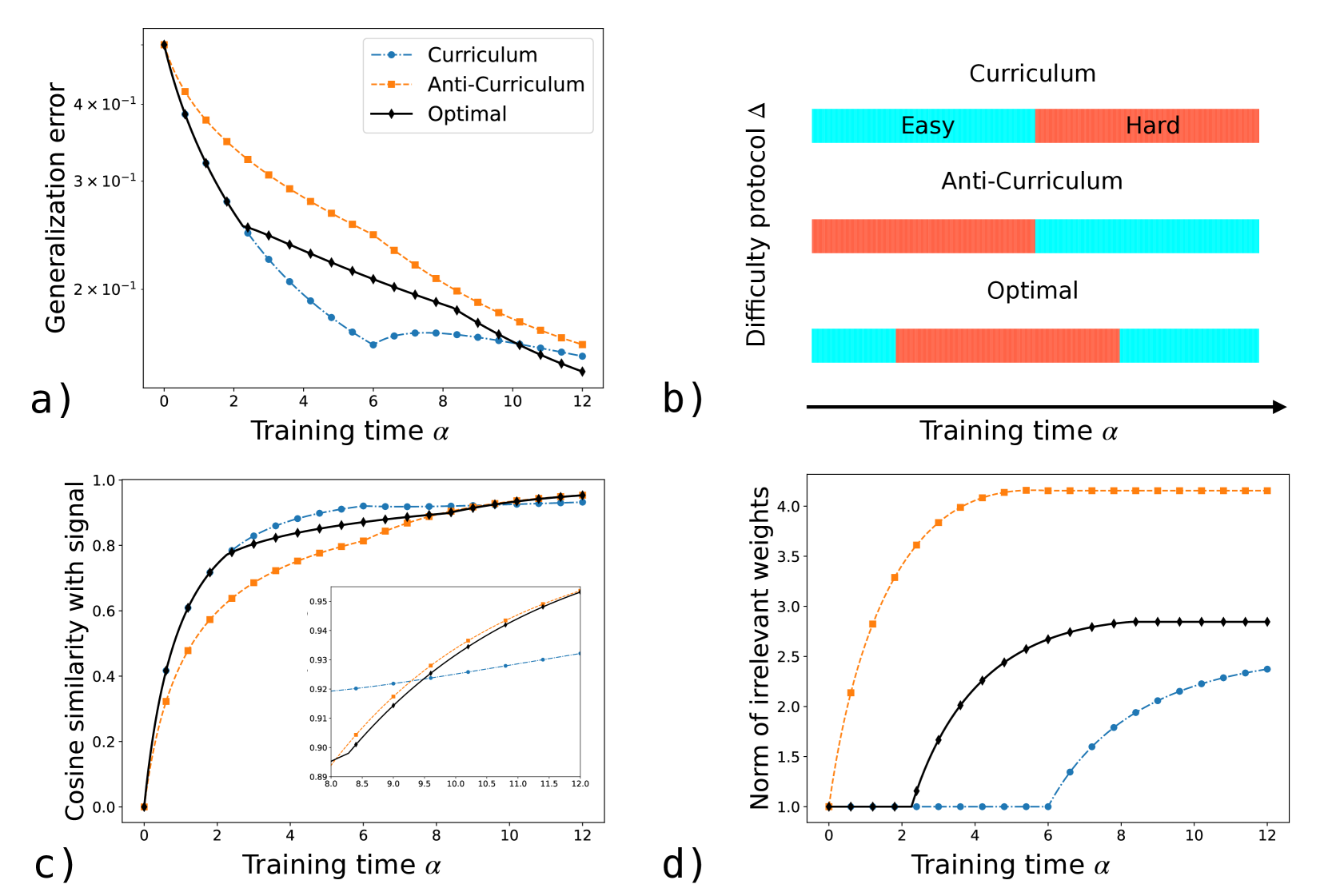
The image is a composite figure containing four subplots (labeled a, b, c, d) that analyze and compare three different training protocols—Curriculum, Anti-Curriculum, and Optimal—across various metrics over training time (α). The figure appears to be from a machine learning research paper investigating the effects of data presentation order on model performance and internal representations.
### Components/Axes
The figure is divided into four quadrants:
* **Top-Left (a):** A line chart plotting "Generalization error" (logarithmic y-axis) vs. "Training time α" (linear x-axis).
* **Top-Right (b):** A horizontal bar chart illustrating the "Difficulty protocol Δ" over "Training time α".
* **Bottom-Left (c):** A line chart plotting "Cosine similarity with signal" (linear y-axis) vs. "Training time α", containing an inset zoom.
* **Bottom-Right (d):** A line chart plotting "Norm of irrelevant weights" (linear y-axis) vs. "Training time α".
**Common Legend (applies to plots a, c, d):**
* **Curriculum:** Blue dashed line with circle markers.
* **Anti-Curriculum:** Orange dashed line with square markers.
* **Optimal:** Black solid line with diamond markers.
**Axes Labels and Scales:**
* **X-axis (all plots):** "Training time α", ranging from 0 to 12.
* **Y-axis (Plot a):** "Generalization error", logarithmic scale. Major ticks at 2×10⁻¹, 3×10⁻¹, 4×10⁻¹.
* **Y-axis (Plot c):** "Cosine similarity with signal", linear scale from 0.0 to 1.0.
* **Y-axis (Plot d):** "Norm of irrelevant weights", linear scale from 1.0 to 4.0+.
* **Y-axis (Plot b):** "Difficulty protocol Δ", categorical (Curriculum, Anti-Curriculum, Optimal).
### Detailed Analysis
**Plot a) Generalization Error vs. Training Time**
* **Trend Verification:** All three lines show a decreasing trend, indicating error reduction over training. The Curriculum line decreases most rapidly initially, then plateaus and is overtaken by the Optimal line. The Anti-Curriculum line decreases the slowest but continues a steady decline.
* **Data Points (Approximate):**
* **α=0:** All start at a high error (~5×10⁻¹).
* **α=2:** Curriculum ~2.5×10⁻¹, Optimal ~2.8×10⁻¹, Anti-Curriculum ~3.5×10⁻¹.
* **α=6:** Curriculum reaches a local minimum (~1.5×10⁻¹), then slightly increases. Optimal continues down to ~2.0×10⁻¹. Anti-Curriculum ~2.5×10⁻¹.
* **α=12:** Optimal achieves the lowest error (~1.2×10⁻¹). Curriculum and Anti-Curriculum converge near ~1.4×10⁻¹.
**Plot b) Difficulty Protocol Schematic**
* **Component Isolation:** This diagram defines the three protocols. The x-axis represents training time. Colors indicate task difficulty: **Cyan = Easy**, **Red = Hard**.
* **Curriculum:** Easy tasks first (cyan bar from α=0 to ~α=6), then Hard tasks (red bar from ~α=6 to α=12).
* **Anti-Curriculum:** Hard tasks first (red bar from α=0 to ~α=6), then Easy tasks (cyan bar from ~α=6 to α=12).
* **Optimal:** A mixed schedule. Starts with a short Easy phase (cyan, α=0 to ~α=2), followed by a long Hard phase (red, ~α=2 to ~α=8), and ends with another Easy phase (cyan, ~α=8 to α=12).
**Plot c) Cosine Similarity with Signal vs. Training Time**
* **Trend Verification:** All lines increase, indicating the model's learned representation becomes more aligned with the true signal over time. The inset shows a late-stage crossover.
* **Data Points (Approximate):**
* **α=0:** All start at 0.0.
* **α=2:** Curriculum ~0.7, Optimal ~0.65, Anti-Curriculum ~0.5.
* **α=6:** Curriculum ~0.9, Optimal ~0.85, Anti-Curriculum ~0.8.
* **α=12 (Main Plot):** Curriculum and Optimal converge near ~0.95. Anti-Curriculum is slightly lower, ~0.93.
* **Inset (α=8 to 12):** Provides a zoomed view. At α=8, Curriculum (~0.92) is highest. By α=12, Optimal (~0.95) has slightly surpassed Curriculum (~0.94), with Anti-Curriculum (~0.93) lowest.
**Plot d) Norm of Irrelevant Weights vs. Training Time**
* **Trend Verification:** This measures the magnitude of weights not contributing to the signal. Anti-Curriculum rises sharply and plateaus high. Optimal rises later to a medium plateau. Curriculum stays low the longest before a late, moderate rise.
* **Data Points (Approximate):**
* **α=0-2:** All norms are at baseline (~1.0).
* **Anti-Curriculum:** Begins rising sharply at α=1, plateaus near 4.2 by α=6.
* **Optimal:** Begins rising at α=2, plateaus near 2.8 by α=8.
* **Curriculum:** Remains near 1.0 until α=6, then rises to plateau near 2.4 by α=10.
### Key Observations
1. **Performance Crossover:** While the Curriculum protocol (easy-to-hard) leads to the fastest initial drop in generalization error (Plot a) and fastest gain in signal similarity (Plot c), the Optimal mixed schedule ultimately achieves the lowest final error.
2. **Protocol Impact on Internal Representation:** The Anti-Curriculum (hard-to-easy) protocol results in a significantly larger norm for irrelevant weights (Plot d), suggesting the model allocates more capacity to noise when faced with difficult tasks early in training.
3. **Late-Stage Dynamics:** The inset in Plot c reveals a subtle but important crossover where the Optimal protocol's representation quality surpasses the Curriculum's in the final stages of training.
4. **Schematic Clarity:** Plot b provides a clear visual definition of the experimental conditions, essential for interpreting the quantitative results in the other panels.
### Interpretation
This figure presents a Peircean investigation into the **causal relationship** between training data scheduling (the **sign** or protocol) and model learning outcomes (the **objects** of error, similarity, and weight norms). The data suggests that the order of task difficulty is not merely a heuristic but a critical factor shaping the learning trajectory.
* **Curriculum Learning (Easy→Hard)** acts as a strong **index** for rapid initial learning, guiding the model efficiently toward a good solution. However, it may lead to premature convergence or suboptimal final representations, as hinted by the plateau in error and the late crossover in similarity.
* **Anti-Curriculum Learning (Hard→Easy)** appears to be a **symbol** of inefficient learning. Starting with hard tasks forces the model to develop complex, potentially noisy representations early (high irrelevant weight norm), which then must be corrected, resulting in slower overall progress.
* **The Optimal Schedule** represents a **rheme** or hypothesis about an ideal balance. Its pattern (Easy→Hard→Easy) suggests a beneficial structure: an initial easy phase for warm-up, a core hard phase for capacity building, and a final easy phase for refinement and consolidation. This schedule achieves the best final generalization, implying that strategic "scaffolding" and "consolidation" phases are key.
The anomaly is the Curriculum's early lead in similarity (Plot c) despite not having the lowest final error. This indicates that alignment with the signal alone is insufficient for optimal generalization; the management of irrelevant parameters (Plot d) is equally crucial. The figure collectively argues for principled, dynamically adjusted training protocols over simple monotonic difficulty schedules.
DECODING INTELLIGENCE...