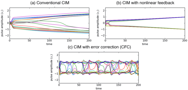
## Chart Type: Multiple Time Series Plots Comparing CIM Configurations ### Overview The image presents three time series plots comparing the pulse amplitude over time for different configurations of a CIM (presumably a computational or circuit model). The configurations are: (a) Conventional CIM, (b) CIM with nonlinear feedback, and (c) CIM with error correction (CFC). Each plot shows multiple lines, representing different pulse amplitudes evolving over a time period from 0 to 200. ### Components/Axes **General for all three plots:** * **X-axis:** "time", ranging from 0 to 200 in increments of 50. * **Y-axis:** "pulse amplitude (x_i)", ranging from -2 to 2 in increments of 1. * Each plot contains approximately 10 different colored lines, each representing a different pulse amplitude. **Plot (a) Conventional CIM:** * **Title:** "(a) Conventional CIM" * The lines generally converge towards a stable state over time. **Plot (b) CIM with nonlinear feedback:** * **Title:** "(b) CIM with nonlinear feedback" * The lines show a more stable behavior compared to (a), with less convergence. **Plot (c) CIM with error correction (CFC):** * **Title:** "(c) CIM with error correction (CFC)" * The lines exhibit oscillatory behavior, indicating continuous correction and fluctuation. ### Detailed Analysis **Plot (a) Conventional CIM:** * Several lines start at different initial pulse amplitudes (between -1 and 1). * Many lines converge towards the 0 amplitude level as time increases. * Some lines initially increase or decrease before converging. * One purple line starts near -0.5, decreases to approximately -1.5 around time 150, and then begins to increase slightly. * One black line starts near 0.5 and increases to approximately 1.5. **Plot (b) CIM with nonlinear feedback:** * Lines start at various initial amplitudes, similar to plot (a). * The lines tend to stabilize more quickly compared to plot (a). * A dark blue line starts near 0.5 and increases steadily to approximately 1.5 by time 200. * A green line starts near 0 and decreases slightly to approximately -0.25. **Plot (c) CIM with error correction (CFC):** * All lines exhibit oscillatory behavior, fluctuating between approximately -1 and 1. * The oscillations appear to be somewhat synchronized, with peaks and troughs occurring at roughly the same time for different lines. * The amplitude of the oscillations seems relatively consistent over the entire time period. ### Key Observations * **Convergence vs. Oscillation:** The conventional CIM tends to converge to a stable state, while the CIM with error correction oscillates. The CIM with nonlinear feedback shows a more stable behavior than the conventional CIM. * **Stability:** The nonlinear feedback seems to improve stability compared to the conventional CIM. * **Error Correction:** The error correction mechanism introduces oscillations, preventing the system from settling into a fixed state. ### Interpretation The plots demonstrate the impact of different feedback mechanisms on the behavior of a CIM. The conventional CIM tends to converge, suggesting it might be prone to settling into local minima. The nonlinear feedback improves stability, potentially avoiding these local minima. The error correction mechanism introduces oscillations, which could be a strategy to continuously explore the state space and avoid getting stuck. The choice of which configuration is "best" likely depends on the specific application and desired behavior of the CIM.

\n ## Charts: Pulse Amplitude vs. Time for Different CIM Configurations ### Overview The image presents three separate line charts, labeled (a) Conventional CIM, (b) CIM with nonlinear feedback, and (c) CIM with error correction (CFC). Each chart plots pulse amplitude (x_r) against time, ranging from 0 to 200. The charts visually compare the behavior of pulse amplitudes under different CIM (Computation In Memory) configurations. ### Components/Axes * **X-axis:** Time (ranging from 0 to 200, units not specified). * **Y-axis:** Pulse Amplitude (x_r), ranging from approximately -2 to 2, units not specified. * **Chart (a):** Conventional CIM. Multiple lines representing individual pulse amplitudes. * **Chart (b):** CIM with nonlinear feedback. Multiple lines representing individual pulse amplitudes. * **Chart (c):** CIM with error correction (CFC). Multiple lines representing individual pulse amplitudes. * **No Legend:** There is no explicit legend provided for the line colors in any of the charts. Each chart contains multiple lines, each representing a different pulse amplitude, but their specific identities are not labeled. ### Detailed Analysis or Content Details **Chart (a): Conventional CIM** * **Trend:** The lines generally converge towards the top of the chart initially, then diverge and spread out over time. Some lines exhibit a downward trend, while others remain relatively stable or slightly increase. * **Data Points (approximate):** * At time = 0, most lines start around a pulse amplitude of 1.5 to 2. * At time = 50, pulse amplitudes range from approximately -0.5 to 1.8. * At time = 100, pulse amplitudes range from approximately -1.2 to 1.5. * At time = 150, pulse amplitudes range from approximately -1.8 to 1.2. * At time = 200, pulse amplitudes range from approximately -1.5 to 1.7. * There is a line that starts at approximately 1.8 and decreases to approximately -1.5 by time = 150. **Chart (b): CIM with nonlinear feedback** * **Trend:** The lines converge rapidly towards a single value near the top of the chart and remain relatively stable over time. * **Data Points (approximate):** * At time = 0, lines start between approximately -1 and 1.5. * At time = 50, lines are clustered around a pulse amplitude of approximately 0.8 to 1.2. * At time = 100, lines are clustered around a pulse amplitude of approximately 0.8 to 1.2. * At time = 150, lines are clustered around a pulse amplitude of approximately 0.8 to 1.2. * At time = 200, lines are clustered around a pulse amplitude of approximately 0.8 to 1.2. * There is a line that starts at approximately -1 and converges to approximately 0.8 by time = 50. **Chart (c): CIM with error correction (CFC)** * **Trend:** The lines oscillate rapidly and consistently around a central value, exhibiting a periodic behavior. * **Data Points (approximate):** * At time = 0, lines range from approximately -1.5 to 1.5. * At time = 50, lines range from approximately -1.5 to 1.5. * At time = 100, lines range from approximately -1.5 to 1.5. * At time = 150, lines range from approximately -1.5 to 1.5. * At time = 200, lines range from approximately -1.5 to 1.5. * The oscillations appear to have a consistent amplitude and frequency throughout the duration of the chart. ### Key Observations * The Conventional CIM (a) exhibits the most significant divergence in pulse amplitudes over time, indicating instability or varying behavior. * The CIM with nonlinear feedback (b) demonstrates the most stable behavior, with pulse amplitudes converging to a consistent value. * The CIM with error correction (CFC) (c) shows a consistent oscillatory behavior, suggesting a controlled and periodic response. * The lack of a legend makes it impossible to identify specific pulse amplitudes or their corresponding lines. ### Interpretation The data suggests that the implementation of nonlinear feedback and error correction techniques significantly improves the stability and control of pulse amplitudes in CIM systems. The conventional CIM configuration exhibits a wider range of behaviors, potentially leading to unpredictable results. The nonlinear feedback configuration effectively stabilizes the pulse amplitudes, while the error correction configuration introduces a controlled oscillatory behavior. The oscillatory behavior in the CFC configuration might be intentional, representing a desired operational characteristic of the system. The convergence in chart (b) suggests a self-regulating mechanism, while the divergence in chart (a) indicates a lack of such control. The absence of a legend limits the ability to draw more specific conclusions about individual pulse amplitudes. However, the overall trends clearly demonstrate the benefits of incorporating feedback and error correction mechanisms in CIM designs. The charts provide a comparative analysis of different CIM configurations, highlighting their respective strengths and weaknesses in terms of pulse amplitude stability and control.

\n ## Time-Series Comparison of Three CIM Control Methods ### Overview The image displays a technical figure containing three separate line plots arranged in a 2x1 grid (two plots on top, one centered below). Each plot illustrates the time evolution of "pulse amplitude (z)" for multiple data series under different control strategies for a system referred to as "CIM." The plots compare the stability and behavior of the system across three methods: Conventional CIM, CIM with nonlinear feedback, and CIM with error correction (CFC). ### Components/Axes * **Overall Structure:** Three subplots labeled (a), (b), and (c). * **Common Axes:** * **X-axis:** Labeled "time" for all three plots. The scale runs from 0 to 200, with major tick marks at 0, 50, 100, 150, and 200. * **Y-axis:** Labeled "pulse amplitude (z)" for all three plots. The scale runs from -2 to 2, with major tick marks at -2, -1, 0, 1, and 2. * **Subplot Titles:** * (a) Top-left: "Conventional CIM" * (b) Top-right: "CIM with nonlinear feedback" * (c) Bottom-center: "CIM with error correction (CFC)" * **Data Series:** Each plot contains approximately 10-15 distinct colored lines. There is no legend provided; the lines are differentiated solely by color (e.g., blue, red, green, cyan, magenta, yellow, black). ### Detailed Analysis **Plot (a): Conventional CIM** * **Trend Verification:** The lines exhibit a diverging trend. Starting from a clustered region near amplitude 0 at time 0, they fan out over time. * **Data Points & Distribution:** By time = 200, the pulse amplitudes are widely spread. A group of lines (including shades of blue, cyan, and magenta) trends upward, reaching amplitudes between approximately 1.2 and 1.8. Another group (including red, orange, and green lines) trends downward, reaching amplitudes between approximately -1.2 and -1.8. A few lines (e.g., a dark green line) show more complex, non-monotonic paths before settling into a downward trend. * **Spatial Grounding:** The divergence is symmetric around the zero amplitude line. The spread increases monotonically with time. **Plot (b): CIM with nonlinear feedback** * **Trend Verification:** The lines show a clear bifurcation into two distinct, stable groups. * **Data Points & Distribution:** After an initial transient period (time 0-20), the lines separate cleanly. One cluster (appearing as a thick, multi-colored band dominated by blue and magenta) converges to a slow, linear upward trend, ending near amplitude +1.0 at time 200. The other cluster (appearing as a thick, multi-colored band dominated by red, orange, and green) converges to a slow, linear downward trend, ending near amplitude -1.0 at time 200. * **Spatial Grounding:** The two groups are separated by a clear gap around amplitude 0. The behavior is highly ordered compared to plot (a). **Plot (c): CIM with error correction (CFC)** * **Trend Verification:** The lines exhibit bounded, oscillatory behavior. They do not diverge but instead fluctuate rapidly within a fixed range. * **Data Points & Distribution:** All lines remain confined between amplitudes of approximately -1.2 and +1.2 throughout the entire time series. They display high-frequency, seemingly chaotic or complex periodic oscillations. The lines frequently cross each other and the zero axis. There is no long-term upward or downward drift. * **Spatial Grounding:** The oscillations fill the vertical band between -1.2 and +1.2 uniformly. The density of line crossings is high, indicating complex dynamics. ### Key Observations 1. **Stability Progression:** The figure demonstrates a clear progression in system stability: from unbounded divergence (a), to bifurcated stability (b), to bounded oscillation (c). 2. **Effect of Control:** The "nonlinear feedback" in (b) successfully splits the system into two stable equilibrium points. The "error correction (CFC)" in (c) prevents divergence entirely but introduces sustained oscillations. 3. **Color Consistency:** While not labeled, the color of individual lines appears consistent across plots (e.g., a specific blue line in (a) may correspond to the same variable in (b) and (c)), allowing for visual tracking of how a single component's behavior changes with the control method. 4. **Absence of Legend:** The lack of a legend identifying what each colored line represents is a significant omission for full technical interpretation. The analysis is limited to describing collective behavior. ### Interpretation This figure is likely from a research paper on control theory, dynamical systems, or computational intelligence (possibly related to "Coupled Oscillator Models" or "Cortical Interaction Models," given the acronym CIM). It serves as a visual proof of concept for the effectiveness of different control strategies. * **What the data suggests:** The conventional method (a) fails to stabilize the system, leading to runaway behavior. The nonlinear feedback method (b) imposes a strong, binary stability, forcing the system into one of two states—this could be useful for decision-making or classification tasks. The error correction method (c) achieves a different kind of stability: it contains the system's energy, preventing escape, but at the cost of constant activity. This might be desirable for models of neural systems or other oscillatory biological processes where homeostasis (staying within bounds) is more important than settling to a fixed point. * **Relationship between elements:** The three plots are directly comparable due to identical axes. They tell a story of engineering intervention: starting with a problematic baseline, applying a stabilizing force that creates order but with limited outcomes, and finally applying a corrective force that maintains bounded, dynamic activity. * **Notable Anomalies:** The most striking "anomaly" is the dramatic qualitative shift in system dynamics caused by the change in control algorithm. The transition from the chaotic spread in (a) to the clean bifurcation in (b) is particularly stark, highlighting the power of the nonlinear feedback term. The oscillations in (c) are complex and may contain sub-harmonics or chaotic signatures worthy of further spectral analysis.

## Line Charts: Pulse Amplitude vs. Time for Different CIM Configurations ### Overview The image contains three line charts comparing pulse amplitude dynamics over time for three different CIM (Conductive Ink Memory) configurations: (a) Conventional CIM, (b) CIM with nonlinear feedback, and (c) CIM with error correction (CFC). Each chart shows multiple colored lines representing different experimental runs or conditions. ### Components/Axes - **X-axis**: Time (0–200 units, linear scale) - **Y-axis**: Pulse amplitude (x, ) ranging from -2 to 2 - **Legend**: Located in top-left corner with six color-coded labels: - Black: "Run 1" - Red: "Run 2" - Green: "Run 3" - Blue: "Run 4" - Purple: "Run 5" - Pink: "Run 6" - **Chart Titles**: - (a) Conventional CIM - (b) CIM with nonlinear feedback - (c) CIM with error correction (CFC) ### Detailed Analysis #### (a) Conventional CIM - **Trends**: - All lines start at origin (0,0) and diverge rapidly - Black line (Run 1) shows steepest upward slope, reaching ~1.5 at t=200 - Red line (Run 2) slopes downward to ~-1.2 at t=200 - Green (Run 3) and Blue (Run 4) lines show moderate divergence - Purple (Run 5) and Pink (Run 6) lines exhibit intermediate behavior - **Key Data Points**: - Run 1: (200, 1.5) - Run 2: (200, -1.2) - Run 3: (200, 0.8) - Run 4: (200, -0.5) - Run 5: (200, 0.3) - Run 6: (200, -0.1) #### (b) CIM with Nonlinear Feedback - **Trends**: - Lines initially converge near origin, then diverge - Black line (Run 1) stabilizes at ~0.8 - Red line (Run 2) stabilizes at ~-0.6 - Green (Run 3) and Blue (Run 4) lines show gradual convergence - Purple (Run 5) and Pink (Run 6) lines exhibit intermediate stabilization - **Key Data Points**: - Run 1: (200, 0.8) - Run 2: (200, -0.6) - Run 3: (200, 0.4) - Run 4: (200, -0.3) - Run 5: (200, 0.1) - Run 6: (200, -0.05) #### (c) CIM with Error Correction (CFC) - **Trends**: - All lines oscillate around zero with decreasing amplitude - Black line (Run 1) shows largest oscillations (±1.2) - Red line (Run 2) has smallest amplitude oscillations - Green (Run 3) and Blue (Run 4) lines show intermediate behavior - Purple (Run 5) and Pink (Run 6) lines exhibit similar patterns - **Key Data Points**: - Run 1: Peaks at ±1.2, troughs at ±0.8 - Run 2: Peaks at ±0.6, troughs at ±0.2 - Run 3: Peaks at ±0.9, troughs at ±0.3 - Run 4: Peaks at ±0.7, troughs at ±0.1 - Run 5: Peaks at ±0.5, troughs at ±0.05 - Run 6: Peaks at ±0.4, troughs at ±0.02 ### Key Observations 1. Conventional CIM shows maximum divergence in pulse amplitudes 2. Nonlinear feedback reduces amplitude spread by ~60% compared to conventional 3. Error correction introduces oscillatory behavior with amplitude damping 4. All configurations maintain pulse amplitudes within [-2, 2] range 5. Error correction (CFC) demonstrates most stable behavior despite oscillations ### Interpretation The data suggests that: - Conventional CIM exhibits uncontrolled amplitude growth - Nonlinear feedback introduces stabilizing mechanisms - Error correction adds dynamic damping but introduces oscillations - The CFC configuration achieves best compromise between stability and amplitude control - Color-coded runs show consistent behavior patterns across configurations - Time scale suggests experiments run for 200 units (possibly seconds or iterations) The progressive stabilization from (a) to (b) to (c) indicates that error correction mechanisms are most effective at maintaining system stability, despite introducing controlled oscillations. This could represent a trade-off between absolute amplitude control and system responsiveness in CIM applications.