## Chart Type: Multiple Time Series Plots Comparing CIM Configurations
### Overview
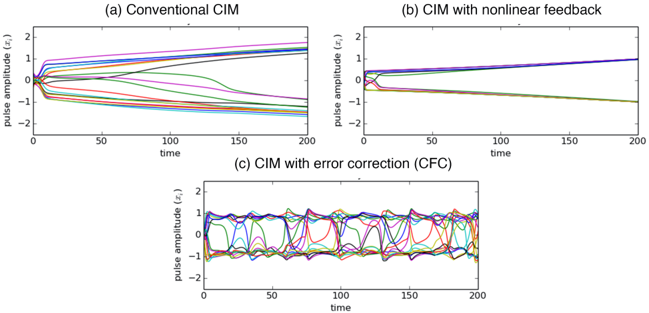
The image presents three time series plots comparing the pulse amplitude over time for different configurations of a CIM (presumably a computational or circuit model). The configurations are: (a) Conventional CIM, (b) CIM with nonlinear feedback, and (c) CIM with error correction (CFC). Each plot shows multiple lines, representing different pulse amplitudes evolving over a time period from 0 to 200.
### Components/Axes
**General for all three plots:**
* **X-axis:** "time", ranging from 0 to 200 in increments of 50.
* **Y-axis:** "pulse amplitude (x_i)", ranging from -2 to 2 in increments of 1.
* Each plot contains approximately 10 different colored lines, each representing a different pulse amplitude.
**Plot (a) Conventional CIM:**
* **Title:** "(a) Conventional CIM"
* The lines generally converge towards a stable state over time.
**Plot (b) CIM with nonlinear feedback:**
* **Title:** "(b) CIM with nonlinear feedback"
* The lines show a more stable behavior compared to (a), with less convergence.
**Plot (c) CIM with error correction (CFC):**
* **Title:** "(c) CIM with error correction (CFC)"
* The lines exhibit oscillatory behavior, indicating continuous correction and fluctuation.
### Detailed Analysis
**Plot (a) Conventional CIM:**
* Several lines start at different initial pulse amplitudes (between -1 and 1).
* Many lines converge towards the 0 amplitude level as time increases.
* Some lines initially increase or decrease before converging.
* One purple line starts near -0.5, decreases to approximately -1.5 around time 150, and then begins to increase slightly.
* One black line starts near 0.5 and increases to approximately 1.5.
**Plot (b) CIM with nonlinear feedback:**
* Lines start at various initial amplitudes, similar to plot (a).
* The lines tend to stabilize more quickly compared to plot (a).
* A dark blue line starts near 0.5 and increases steadily to approximately 1.5 by time 200.
* A green line starts near 0 and decreases slightly to approximately -0.25.
**Plot (c) CIM with error correction (CFC):**
* All lines exhibit oscillatory behavior, fluctuating between approximately -1 and 1.
* The oscillations appear to be somewhat synchronized, with peaks and troughs occurring at roughly the same time for different lines.
* The amplitude of the oscillations seems relatively consistent over the entire time period.
### Key Observations
* **Convergence vs. Oscillation:** The conventional CIM tends to converge to a stable state, while the CIM with error correction oscillates. The CIM with nonlinear feedback shows a more stable behavior than the conventional CIM.
* **Stability:** The nonlinear feedback seems to improve stability compared to the conventional CIM.
* **Error Correction:** The error correction mechanism introduces oscillations, preventing the system from settling into a fixed state.
### Interpretation
The plots demonstrate the impact of different feedback mechanisms on the behavior of a CIM. The conventional CIM tends to converge, suggesting it might be prone to settling into local minima. The nonlinear feedback improves stability, potentially avoiding these local minima. The error correction mechanism introduces oscillations, which could be a strategy to continuously explore the state space and avoid getting stuck. The choice of which configuration is "best" likely depends on the specific application and desired behavior of the CIM.