## Histogram: Centrality Measures Distribution
### Overview
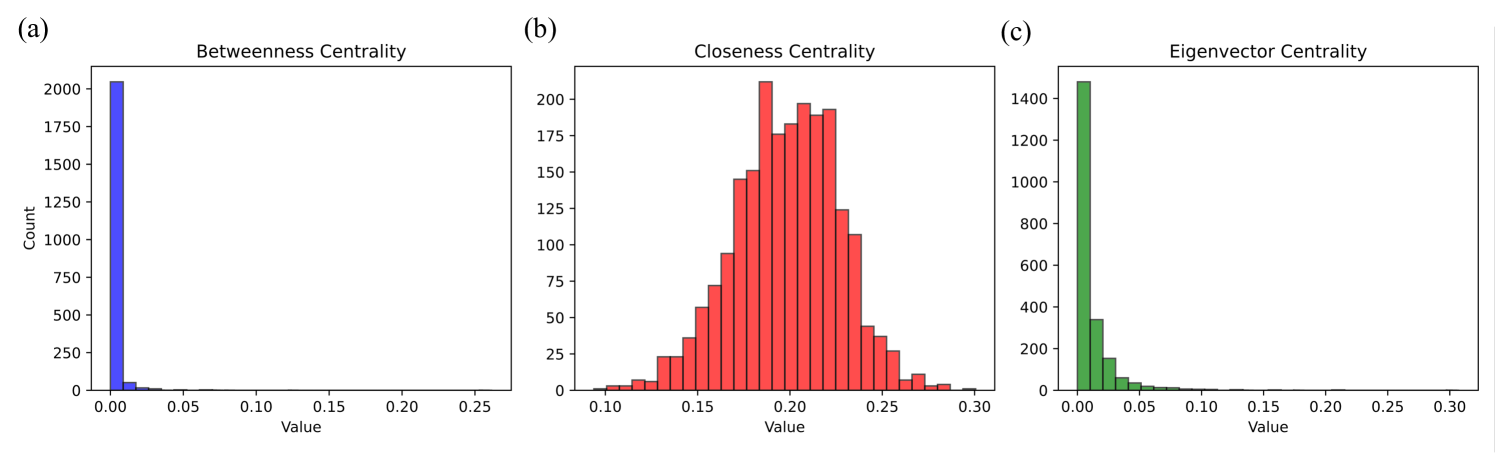
The image presents three histograms, each displaying the distribution of a different centrality measure: Betweenness Centrality, Closeness Centrality, and Eigenvector Centrality. The histograms are arranged horizontally, labeled (a), (b), and (c) respectively. Each histogram plots the count of nodes (y-axis) against the centrality value (x-axis).
### Components/Axes
* **Titles:**
* (a) Betweenness Centrality
* (b) Closeness Centrality
* (c) Eigenvector Centrality
* **X-axis (Value):**
* All three histograms share the same x-axis scale, ranging from 0.00 to 0.30, with tick marks at intervals of 0.05.
* **Y-axis (Count):**
* Histogram (a) ranges from 0 to 2000, with tick marks at intervals of 250.
* Histogram (b) ranges from 0 to 200, with tick marks at intervals of 25.
* Histogram (c) ranges from 0 to 1400, with tick marks at intervals of 200.
* **Colors:**
* Betweenness Centrality (a) is represented in blue.
* Closeness Centrality (b) is represented in red.
* Eigenvector Centrality (c) is represented in green.
### Detailed Analysis
* **Betweenness Centrality (a):**
* The distribution is heavily skewed to the left.
* A large number of nodes have a betweenness centrality value close to 0.
* The count at value 0.00 is approximately 2050.
* The count at value 0.05 is approximately 100.
* The count at value 0.10 is approximately 25.
* The count at value 0.15 is approximately 10.
* The count at value 0.20 is approximately 5.
* The count at value 0.25 is approximately 2.
* **Closeness Centrality (b):**
* The distribution is approximately normal, centered around 0.20.
* The count at value 0.10 is approximately 5.
* The count at value 0.15 is approximately 75.
* The count at value 0.20 is approximately 200.
* The count at value 0.25 is approximately 50.
* The count at value 0.30 is approximately 5.
* **Eigenvector Centrality (c):**
* The distribution is heavily skewed to the left, similar to Betweenness Centrality.
* A large number of nodes have an eigenvector centrality value close to 0.
* The count at value 0.00 is approximately 1450.
* The count at value 0.05 is approximately 350.
* The count at value 0.10 is approximately 50.
* The count at value 0.15 is approximately 10.
* The count at value 0.20 is approximately 5.
* The count at value 0.25 is approximately 2.
* The count at value 0.30 is approximately 1.
### Key Observations
* Betweenness and Eigenvector Centrality distributions are highly skewed, indicating that most nodes have very low centrality values for these measures.
* Closeness Centrality exhibits a more normal distribution, suggesting a more even distribution of closeness centrality values among the nodes.
* The scales of the y-axes differ significantly, reflecting the different ranges of counts for each centrality measure.
### Interpretation
The histograms illustrate the distribution of three different centrality measures within a network. The skewness observed in the Betweenness and Eigenvector Centrality distributions suggests that only a small fraction of nodes have high influence or control over the network's communication pathways (Betweenness) or are highly connected to other influential nodes (Eigenvector). In contrast, the more normal distribution of Closeness Centrality indicates that nodes are, on average, relatively close to all other nodes in the network.
These distributions can provide insights into the network's structure and dynamics. For example, a network with a highly skewed Betweenness Centrality distribution might be vulnerable to disruptions if the few nodes with high betweenness are removed. Similarly, a network with a more evenly distributed Closeness Centrality might be more resilient to such disruptions.